Opening the book…
This exercise will focus on the second step of the process that was outlined at the end of the preceding section, namely creating one or more artificial waveforms that will be used to assess waveform distortion.
ERPLAB Studio contains a tool for creating these waveforms that you can access via the Create Artificial ERP Waveform panel in the ERP tab (or via scripts). This tool allows you to create an artificial waveform with a small number of parameters and overlay this with a real waveform that provides an approximation of the true effect. Let’s take a look at how this works, first for the N170 component and then for the N400 component. Then we’ll consider the question of how you can make an educated guess about what the true effect will look like for less well-studied components.
Start by clicking the Reset button under the lower right corner of the plot region and then clicking Reset ERPLAB Studio in the window that appears. Then load the ERPset named N170.erp using the ERPsets panel and select only the PO8 electrode site (channel 26) from the Bin & Channel Selection panel. The result should look like Screenshot 4.32.
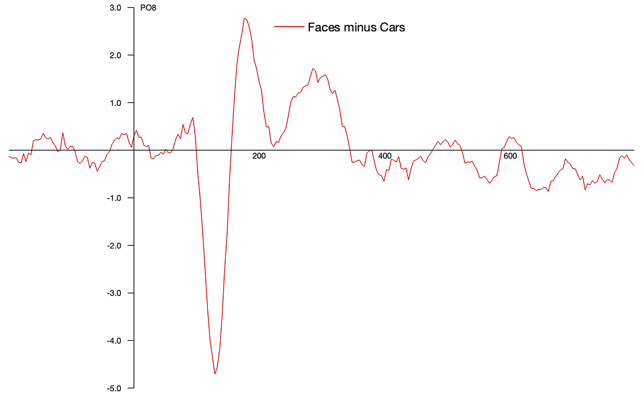
You are now looking at the grand average N170 component from the ERP CORE (Kappenman et al., 2021). In this experiment, participants saw faces, cars, scrambled faces, and scrambled cars, and on each trial they pressed a button to indicate whether or not the stimulus was scrambled (irrespective of whether it was a face or a car). In the ERPset you just loaded, the N170 component was isolated by constructing a faces-minus-cars difference wave. This is a common approach, which subtracts away any brain activity that is equivalent for faces and cars, leaving the differential activity. This differential activity is mainly the N170 component (which is primarily the additional activity associated with face processing), although there are some smaller positive components after the N170.
Now we’re going to create an artificial waveform that closely resembles the N170 component (without the subsequent positivities). Go to the Create Artificial ERP Waveforms panel, and check the box labeled Compare with Real Data near the top of the panel. We have only one ERPset, so you can leave the ERPset box set to 1. We want to select the PO8 channel, so click the Browse button next to the Channel box, click on the P08 channel (which is channel 26), and click OK. You should now see 26 in the Channel box. There is only one bin, so you can leave the Bin box at 1. You should see something like Screenshot 4.33.

The real N170 grand average should be shown in red, and the current artificial ERP waveform should be shown in blue. It’s obviously not a good match, because the artificial waveform is a positivity peaking around 100 ms. Let’s change the artificial waveform so that it’s a negativity that more closely matches the N170, with an amplitude of approximately -4.5 µV and a latency of approximately 170 ms. Within the panel, go to the section labeled Basic Function for Simulation and change the Peak amplitude to -4.5 and the Gaussian mean to 170, with the SD set to 50. This should create an artificial waveform with an amplitude of -4.5 µV and a latency of 170 ms. As shown in Screenshot 4.34, the match is better, although the artificial waveform is too wide and it peaks too late.

As you can probably tell, this tool is using a Gaussian (normal distribution) function to simulate the waveform. Try playing around with the latency (the mean of the Gaussian), the width (the standard deviation or SD of the Gaussian) and the peak amplitude (the height of the Gaussian) to get it to better match the observed N170.
In our journal article, we found the best fit with a Peak amplitude of -4.6, a Gaussian mean of 129 ms, and an SD of 14 (see Screenshot 4.35). It’s not perfect, and it doesn’t attempt to account for the positive waves that follow the N170, but it’s a pretty good match to the N170. Once you are satisfied with the match between your simulated N170 and the grand average, click the Create ERPset button at the bottom of the panel, and name the new ERPset Simulated N170. You should also save the ERPset to the folder for this exercise, because you will need it later.

Now we’re going to create a simulated N400 to match the grand average from the ERP CORE N400 experiment. Start by clearing the loaded ERPsets from the ERPsets panel and then using this panel to load the file named N400.erp. This ERPset has one bin corresponding to the N400 difference wave (unrelated targets minus related targets). Select the CPz channel (Channel 14) from the Bin & Channel Selection panel. You should see something like Screenshot 4.36, with a large N400 peaking at approximately 350 ms.

Now go to the Create Artificial ERP Waveforms panel, make sure the box labeled Compare with Real Data is checked, and set the ERPset box to 1. We want to select the CPz channel (because this is where the N400 is largest), so click the Browse button next to the Channel box, click on the CPz channel, and click OK. You should now see 14 in the Channel box. There is only one bin, so you can leave the Bin box at 1. Now go to the section of the panel labeled Basic Function for Simulation and change the Peak amplitude to -9.65, the Gaussian mean to 350, and the SD to 65. You should see something like Screenshot 4.37.

Although the artificial waveform is a pretty good match for the part of the waveform prior to the peak, it’s a poor match for the part of the waveform after the peak. This is because the artificial waveform is a mirror-symmetrical Gaussian function, whereas the N400 difference wave has a rightward skew. This kind of skew is found in many higher-level ERP components (for an explanation, see Chapter 9 in Luck, 2014).
To better fit skewed waveforms, ERPLAB uses an ExGaussian function to create artificial ERP waveforms. This function is a convolution of an exponential function (which can have different amounts of skew) and the symmetrical Gaussian function. The skewness of the exponential function is determined by the tau (time constant) parameter. Up until this point, we’ve used a value of zero for tau, resulting in a pure Gaussian function. But now we need to use a nonzero tau value to simulate the skewed N400 difference wave.
To do this, go to the section of the panel labeled Basic Function for Simulation and enter a value of 1400 in the Exponential tau box. This gives us approximately the right amount of skewness, but now the latency of the artificial waveform has shifted rightward. To account for this, change the Gaussian mean to 280 ms. You should now see a pretty good match, as shown in Screenshot 4.38. To create an ERPset with this simulated N400, click the Create ERPset button at the bottom of the panel, name the new ERPset Simulated N400, and save it to disk.

You’ve now seen the process of creating artificial waveforms that simulate two different ERP components. In the next exercise, you’ll apply several different filters to these waveforms and quantify the amount of waveform distortion. But I suspect that you have some questions about the process of creating the artificial waveforms, which I will try to answer here.
First, you may be wondering what to do if your simulated waveform doesn’t perfectly match the real data. For example, our simulated N170 waveform doesn’t include the positivities that follow the N170 in the grand average, and our simulated N400 waveform doesn’t match the very end of the grand average waveform.
Our goal here is not perfection. We are just trying to figure out a reasonable set of filtering settings that will do a good job of reducing noise without producing too much waveform distortion. The criterion for “too much waveform distortion” is somewhat arbitrary, so perfection is not even well defined. You should also keep in mind that slightly different filter settings will produce only slightly different results, so you don’t need to get the settings exactly right. Your goal is to determine the filter settings that are approximately optimal. So don’t worry if the simulated effect doesn’t perfectly match the grand average waveform.
A second issue arises when the grand average waveform is quite noisy, so you don’t know what the true effect actually looks like. This wasn’t a problem for the ERP CORE experiments, because we had plenty of trials and plenty of participants, and we had hundreds of prior studies to compare our waveforms with. But it’s often a problem if you’re embarking on a new program of research, and you have only one or two somewhat noisy previous studies to rely on. If you’re in this situation, I’d recommend creating multiple simulated waveforms, each reflecting a different plausible estimate of the true effect. You can then choose filter settings that won’t produce unacceptable levels of distortion with any of them.
A third question is what to do when the grand average waveform you are using to estimate the real effect contains multiple components that are each reasonably large. For example, in many oddball paradigms, the P3b is isolated with a rare-minus-frequent difference wave, but there may also be an N2 preceding the P3b in this difference wave. Or you may be in a situation where you can’t even make a difference wave. In these situations, I recommend making multiple artificial waveforms, one for each component. You can then sum these together to make sure that the sum does a good job of matching the combined components in the grand average waveform. Then, you can examine the waveform distortions produced for each component individually and for their sum. This is what we did in Section 4.8 for the combination of the P1, N1, and P2 components. The box below provides concrete information about how to combine the components using eStudio.
Combining simulated ERPsets
Once you have created the individual simulated components in separate ERPsets using the Create Artificial ERP Waveforms panel, you can combine them together into a single ERPset using the Append ERPsets panel. To do this, first select the ERPsets for the simulated components in the ERPsets panel. Then go to the Append ERPsets panel and tell it to append the selected ERPsets. This will create a new ERPset in which each simulated component is in a separate bin. You can then use the Bin Operations panel and write an equation that creates a new bin by summing together the bins for all of the simulated components. For example, when I did this with the simulated P1, N1, and P2 components, the individual components were in bins 1-3, and I used this equation in the Bin Operations panel to combine them together: b4 = b1 + b2 + b3 Label P1+N1+P2
This page titled 4.13: Exercise- Creating artificial waveforms was last modified on Thu, 01 Oct 2026 18:52:59 GMT and is shared under a CC BY-NC 4.0 license and was authored, remixed, and/or curated by Steven J Luck.
The book could not be loaded just now.