4.14: Exercise- Quantifying Waveform Distortion in the Artificial Waveforms

This exercise will focus on the third step of the process that was outlined at the end of Section 4.12, namely quantifying the waveform distortion that occurs when we apply a set of filters to the simulated N170 and N400 waveforms you created in the preceding exercise.

The left portion of Figure 4.11 illustrates this part of the overall process. Once we have the simulated ERP waveform, we loop through a set of candidate filters. For each filter, we apply the filter to the simulated waveform and compute the artifactual peak percentage (APP) to quantify the waveform distortion for that filter. The right portion of Figure 4.11 illustrates the resulting APP values across all the candidate filters. We compare the APP values with our threshold, and the ones that are below the threshold are considered to produce “acceptable” levels of waveform distortion. These are the ones that we will further examine to quantify how they impact the data quality (signal and noise). The ones above the threshold are ruled out. In this example, we will use an APP threshold of 5% for the reasons described in Chapter 4.12.

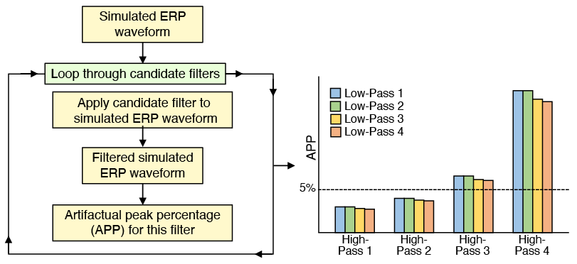
How do you know what set of filters to try? For most cognitive and affective research, I recommend starting with all combinations of the low-pass and high-pass cutoffs shown in Table 4.2. I recommend using a roll-off of 12 dB/octave; we examined steeper roll-offs, and we never found them to be useful for basic filtering (although that might not be true with all types of studies, so you could explore different roll-offs as well as different combinations of low-pass and high-pass cutoffs).

Table 4.2. Initial set of filter cutoffs to assess for most cognitive and affective studies. All 5x5 combinations of these cutoffs should be assessed.

Table 4.2. Initial set of filter cutoffs to assess for most cognitive and affective studies. All 5x5 combinations of these cutoffs should be assessed.

High-pass cutoff	Low-pass cutoff
0.1 Hz	40 Hz
0.5 Hz	30 Hz
1 Hz	20 Hz
2 Hz	10 Hz

If you are looking at short-latency (<100 ms) sensory components, you’ll probably want to shift both the low-pass and high-pass cutoffs to higher values. If you are looking at very slow cognitive and affective components (lasting 500 ms or longer), you’ll probably want to shift the high-pass cutoffs lower but keep the low-pass cutoffs the same.

Once you try these, it should be clear whether you’ve bracketed the range of good candidates (i.e., with some that have too much waveform distortion, and others that don’t improve the signal quality enough). And once you have the right range, you can look at a finer set of gradations within that range (as will be discussed below).

In the present exercise, we will see how ERPLAB Studio can be used to compute the APP values for this set of candidate filters. Start by clicking the Reset button under the lower right corner of the plot region and then clicking Reset ERPLAB Studio in the window that appears. Then load the ERPset named Simulated N170.erp that you created in the preceding exercise (a copy is also present in the Extra Files folder within the folder for the Chapter 14 exercises).

Let’s see what happens with the most extreme filter in our set of candidate filters, with a high-pass cutoff at 2 Hz and a low-pass cutoff at 10 Hz. This filter passes the narrowest range of frequencies, so it’s likely to produce the greatest waveform distortion.

Go to the Filtering panel and select a high-pass cutoff at 2 Hz and a low-pass cutoff at 10 Hz, with a roll-off of 12 dB/octave. Then click Run and name the resulting ERPset Simulated N170_filt2-10. It should look like Screenshot 4.39, with artifactual positive peaks surrounding the negative N170 peak.

The next step is to score the amplitudes of the artifactual peaks along with the true N170 peak. Go to the Measurement Tool panel and set it up to score the peak amplitude of the N170, as shown in Screenshot 4.40. The measurement Type should be Negative Peak Amplitude. The filtered waveform should be ERPset #2, so you can put a 2 in the ERPset field. The ERPset has only 1 bin and 1 channel, so you should put a 1 into the Bin and Channel boxes. A reasonable window for the N170 peak is 100-300 ms, so put 100 300 into the Window box. You can leave the Output box empty, because we’re only getting one value and we can do that easily using the Measurement Tool's preview function. 

To get the N170 peak amplitude score, click the Preview button. You can see that the peak amplitude is -2.059 µV. Click Close to close the preview window and go back to the Measurement Tool panel.

Now score the amplitude of the first artifactual positive peak by changing the Type to Positive Peak Amplitude and changing the Window to 100 200. If you click the Preview button, you can see that the artifactual positive peak has an amplitude of +0.316 µV. Click Close to close this window. The first and second positive peaks are nearly identical, so we only need to score the first one. If you have multiple artifactual peaks, but they have different amplitudes, use the one with the greatest amplitude.

The artifactual peak percentage is simply 100 times the absolute value of the artifactual positive peak's amplitude divided by the absolute value of the N170's peak amplitude: APP = 100 * 0.316 / 2.059 = 15.3%. This is clearly above our threshold of 5%, so this filter produces too much waveform distortion to be considered further.

Now repeat this process with cutoffs of 0.5 Hz and 30 Hz. That is, filter the original Simulated N170 ERPset with these cutoffs and then measure the amplitude of the true N170 peak amplitude and the artifactual positive peak preceding the N170. You should find values of -4.002 µV and +0.100 µV, respectively, which gives us APP = 100 * 0.003 / 4.324 = 2.5%. These filter settings produced only a little bit of waveform distortion, and the APP was under the 5% threshold.

The amplitude of the artifactual positive peak, +0.100 µV, may not seem to match what you saw when you first looked at the waveform (Screenshot 4.41, left). In that waveform, the peak amplitude appears to be about 20% of the way between the baseline and the 1.0 µV marker, which should be an amplitude of about 0.2 µV. This discrepancy is a result of ERPLAB's policies about baseline correction. Filtering the N170 wave created an overall positive offset during the prestimulus period, which you can see when you look at the main eStudio plotting window (and Screenshot 4.41, left). However, the default behavior for the Measurement Tool is to re-baseline the data using the average voltage in the prestimulus period prior to measuring anything. If you look at the waveform in Preview, you will see that it has been re-baselined. This is usually the desired behavior, but it can be overridden by clicking the Baseline button next to the measurement window in the Measurement Tool panel.

If you want to manually re-baseline the data prior to running the Measurement Tool, you can use the Baseline Correction & Linear Detrend panel to perform a baseline correction on the ERPset (see the result of this in Screenshot 4.41, right).

The results so far indicate that a bandpass of 0.5 – 30 Hz is acceptable for the N170 component, whereas a bandpass of 2 – 10 Hz leads to an unacceptable artifactual peak percentage. It's important to realize, however, that the amount of waveform distortion depends on the shape of the component being filtered, not just the filter settings. To see this for yourself, repeat these steps for these two filters with the Simulated N400 ERPset (which you can find in the Extra Files folder). I recommend using a measurement window of 100 300 for the artifactual positive peak and 200 500 for the true N400 peak.

You should find an artifactual positive percentage of 9.76% (100 x 0.737 ÷ 7.555) for the 0.5 – 30 Hz bandpass and 44.2% (100 x 1.173 ÷ 2.653) for the 2 – 10 Hz bandpass. Both of these are well above the 5% threshold, so neither would be an acceptable filter for the N400. This shows why it is important to select filter cutoffs that are appropriate for the specific ERP effects in a given study.

It would take quite a bit of time and effort to repeat this process for all 25 of the cutoff combinations listed in Table 4.2. It could be worthwhile, especially if you're going to run many similar studies and can use the same filter settings for all of them. But the easiest solution in most cases is to write a script that will automatically compute the APP values for every candidate filter. I've created a script named Script1_APP.m for this purpose. You can find it in the folder for this chapter. It creates the simulated N170 and N400 waveforms, filters them, uses the Measurement Tool to get the peak amplitudes of the true and artifactual peaks, and computes the APP. Here's what the output looks like:

bandpass 0.10 to 10.00 Hz: N170 APP = 0.77%, N400 APP = 0.04%
bandpass 0.10 to 20.00 Hz: N170 APP = 0.07%, N400 APP = 0.18%
bandpass 0.10 to 30.00 Hz: N170 APP = 0.08%, N400 APP = 0.21%
bandpass 0.10 to 40.00 Hz: N170 APP = 0.08%, N400 APP = 0.22%
bandpass 0.50 to 10.00 Hz: N170 APP = 2.28%, N400 APP = 9.49%
bandpass 0.50 to 20.00 Hz: N170 APP = 2.56%, N400 APP = 9.72%
bandpass 0.50 to 30.00 Hz: N170 APP = 2.51%, N400 APP = 9.76%
bandpass 0.50 to 40.00 Hz: N170 APP = 2.47%, N400 APP = 9.77%
bandpass 1.00 to 10.00 Hz: N170 APP = 7.24%, N400 APP = 24.84%
bandpass 1.00 to 20.00 Hz: N170 APP = 7.14%, N400 APP = 25.28%
bandpass 1.00 to 30.00 Hz: N170 APP = 6.96%, N400 APP = 25.35%
bandpass 1.00 to 40.00 Hz: N170 APP = 6.83%, N400 APP = 25.37%
bandpass 2.00 to 10.00 Hz: N170 APP = 15.36%, N400 APP = 44.23%
bandpass 2.00 to 20.00 Hz: N170 APP = 15.12%, N400 APP = 44.76%
bandpass 2.00 to 30.00 Hz: N170 APP = 14.79%, N400 APP = 44.85%
bandpass 2.00 to 40.00 Hz: N170 APP = 14.53%, N400 APP = 44.87%

This script would be fairly easy to modify for your own research. You would just update the parameters that control the size, latency, and shape of the components, the filter cutoffs to test, and the time windows used to measure the true and artifactual components.

As you can see from the script's output, most of these filters yield unacceptably high levels of waveform distortion (APP values of >5%). Anything with a high-pass cutoff of >0.5 Hz is unacceptable for the N170, and anything with a high-pass cutoff of > 0.1 Hz is unacceptable for N400. A reasonable next step would be to look at high-pass cutoffs between 0.1 and 1 Hz with a finer granularity (e.g., every 0.1 Hz) to get a more precise idea of the point at which the waveform distortion becomes unacceptable. However, we won't do that here.

The final step, which will be demonstrated in the next section, is to determine how well the various acceptable filters minimize noise. The optimal filter will then be the one that minimizes noise the best while still having an APP of <5%.

---