5.8: Binomial Demonstration

Instructions

This demonstration allows you to explore the binomial distribution. Here you can specify the number of trials (\(N\)) and the proportion of successes (\(p\)). Note that the proportion of successes is sometimes referred to with the Greek letter \(p\); here it will be referred to as \(p\).

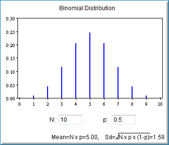
The starting values for \(N\) and \(p\) are \(10\) and \(0.5\). The graph therefore shows the probability of from \(0\) to \(10\) successes out of \(10\) trials. The probability of \(0\) successes is so small that it just barely shows up on the graph. The most likely number of successes is \(5\), which has a probability of about \(0.25\). Naturally, the sum of the probabilities is \(1.0\).

The demonstration also shows the mean and the standard deviation of the binomial distribution.

Illustrated Instructions

The screenshot below shows the binomial demonstration with its default data. You can adjust the number of trials (\(N\)) as well as the proportion of successes (\(p\)).

The example below shows a distribution of \(20\) trials with a probability of success of \(0.7\). Notice that the mean and standard deviation for the distribution are also shown.