From LibreTexts, under CC BY-NC-SA 4.0, as the source states it; its equations are written in TeX, which the PDF shows typeset. This page at LibreTexts.
JASP has two ‘modes’ that allow you to access different options:
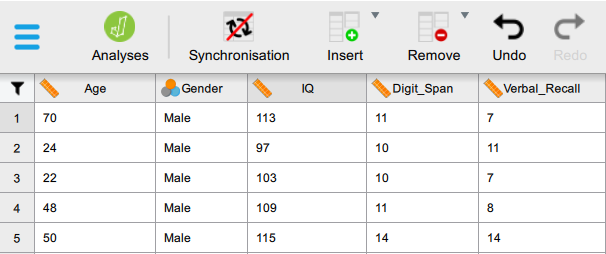
1. Data View Mode – allows you to edit your data; create, modify, and delete variables; compute new variables from existing ones
2. Analysis Mode – allows you to ‘work’ with the data. This includes obtaining descriptive statistics, performing different analyses, and generating tables and graphs.
When working with a dataset you first want to get an overview of the data. For example, what is the distribution of the data? What are the key descriptive statistics that encapsulate this data? All of the tools for analysing your data can be found by clicking on the green Analyses button which will take you out of the ‘Data View Mode’ and into ‘Analysis Mode’.
When you click ‘Analyses’ the menu options at the top change, If you need to go back into ‘Data View Mode’, you simply need to click the Edit Data button which has replaced the ‘Analyses’ button.
Descriptive Statistics
To find the tools for descriptive statistics, plots, and graphs you need to click the Descriptives button which is the first option in the top menu.
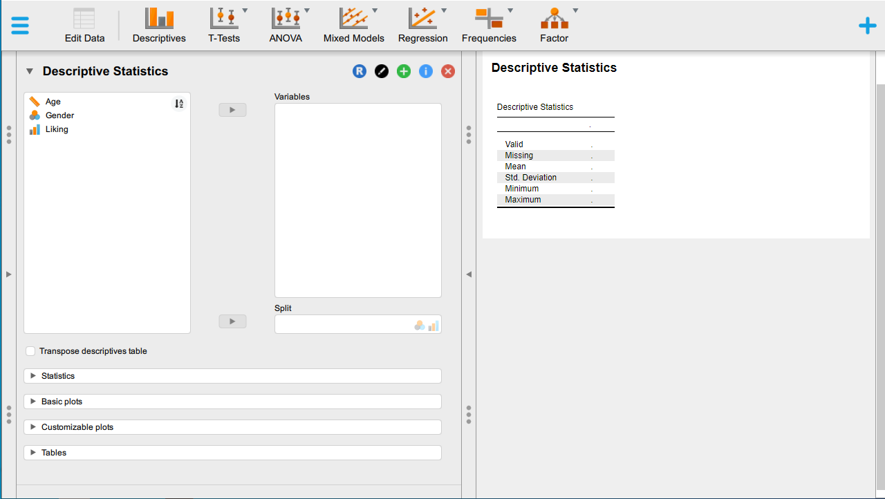
When you click the Descriptives button, a new screen will appear, like so:
Your new screen is now split into two:
Left-hand side has the variables that you can select with a number of expandable menus: ‘Statistics’, ‘Basic plots’, ‘Customizable plots’, and ‘Tables’ (you will need these later).
Right-hand side shows you the output from the options you can select on the left-hand side.
There are two main options for extracting descriptive statistics from your data depending upon the kind of information you want to obtain. These have been explained in the next two sections.
Continuous Variables for a Single Group of Participants
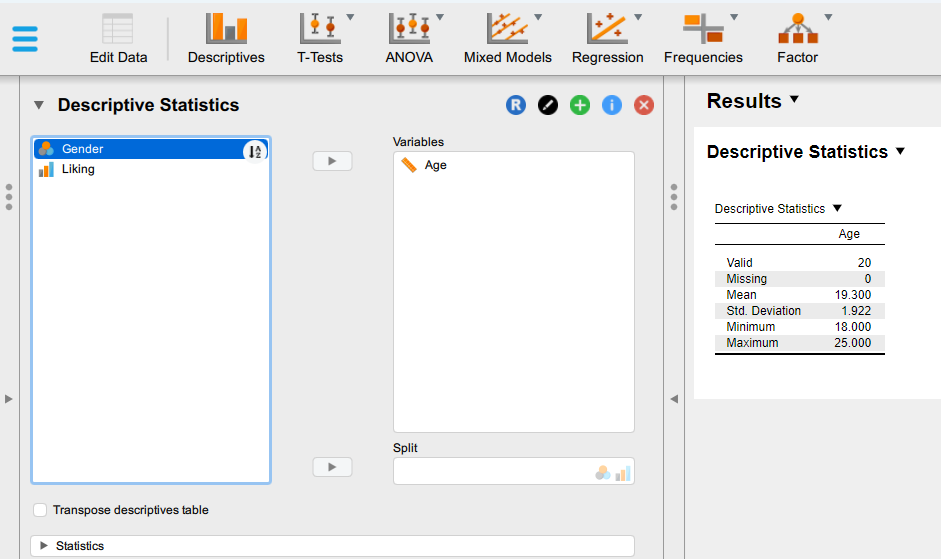
1. Move the continuous variable(s) you are interested in into the Variables box. Continuous (scale) variables are indicated by a ruler symbol.
2. As soon as you move the variable(s) across, the Descriptive Statistics table on the right-hand side of the screen will populate with information (e.g., mean and standard deviation).
Continuous Variables for Different Groups of Participants
1. Move the continuous variable(s) you are interested in into the Variables box.
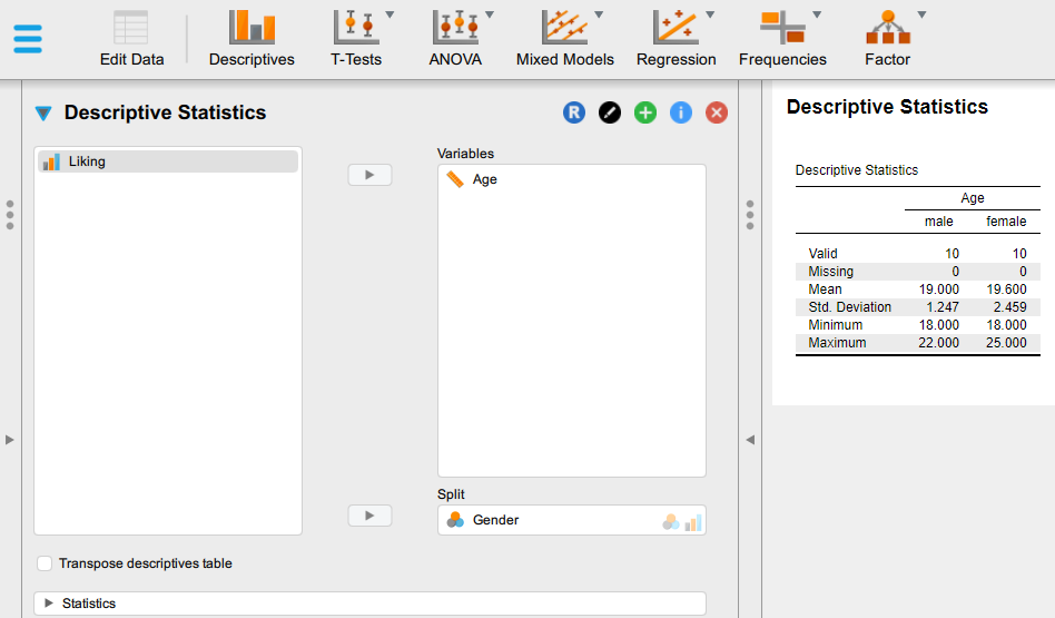
2. Move the categorical variable you want to use to create separate groups into the Split box below Variables. Categorical (nominal) variables are indicated by a Venn diagram symbol.
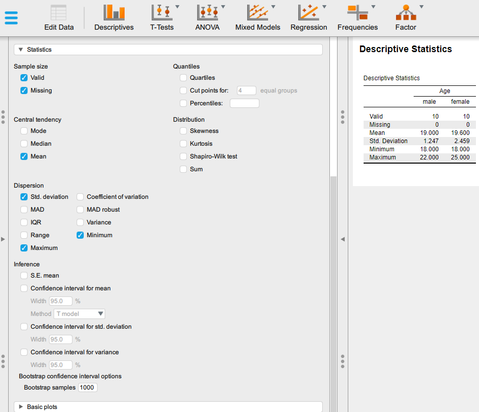
3. As soon as you move the variable(s) across, the Descriptive Statistics table on the right-hand side of the screen will populate with information (e.g., mean and standard deviation for each group of participants).
4. You can change the statistics provided in the Descriptives Statistics table. To do so, click on the Statistics button to expand the menu and select the statistics you wish to see in the table. The most common statistics have already been selected in the screenshot below.
Note:The best thing about JASP is that you can click and unclick as many options as you like! You will be able to see the output from your selected options immediately on the right-hand side of the screen. Feel free to play around and experiment.
Investigating Outliers – Calculating the Z-Score
Before you can start analysing your data, you will need to check some of the most common assumptions for inferential parametric tests. For example, whether there are any outliers (i.e., unusual values) in the data.
In this section, we show you how to detect extreme outliers for continuous variables using z-scores. [1]
How do I do that?
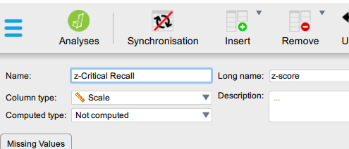
1. Create a new variable next to the variable you want to calculate the z-scores for.
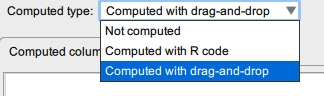
2. Name this variable ‘z-[name of original variable]’, then in the Computed typemenu select ‘Computed with drag-and-drop’.
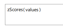
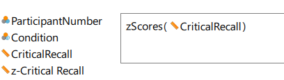
3. Scroll down the menu on the right-hand side of the computed column box until you see zScores(y).
4. Drag and drop zScores(y) into the large box in the centre. Then drag the original variable so that it falls in between the brackets.
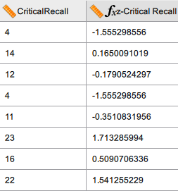
5. The new variable will now be populated with the z-scores.
6. Optional: You can sort the z-scores into descending or ascending order to more easily see extreme values. Remember that outliers can be positive or negative so you should check both ends of the column.
The z-score is a standardised statistic that tells you how many standard deviations away from the mean each data point is. A general rule of thumb is that z-scores above 3 or below -3 are extreme outliers. 3.01: Descriptive Statistics#return-footnote-244-1