4.8: Exercise- Filtering a Series of Impulses (and a Sneaky Introduction to Convolution)
Opening the book…
In the preceding exercise, you learned about the impulse response function of a filter. In the present exercise, we’re going to see how a filter’s impulse response function can be used to understand the effects of the filter on an entire ERP waveform. This exercise is a little long, but it's worth it because by the end you should truly understand how filters work!
To keep things simple, we’re going to use a simplified waveform that contains only a single ERP component (the P1 wave that was combined with the N1 and P2 waves to create the simulated ERP waveform in the previous two exercises). Figure 4.4 shows the P1 waveform, with Panel A showing the usual format and Panel B showing the waveform as a series of impulses.
Figure 4.4. Two ways of drawing the P1 wave, which actually consists of one voltage value every 10 ms (because the sampling rate in this example is 100 Hz). (A) Conventional approach, in which the points are connected with lines to make it look like a continuous waveform. (B) Alternative approach to plotting, in which the voltage at each time point is represented with an impulse so that we can more easily conceptualize the role of the impulse response function in filtering.
The waveform in Figure 4.4 is stored in an ERPset named P1_Separated, which you should load using the ERPsets panel. As shown in Screenshot 4.17, Channel 14 of this ERPset contains the P1 wave. Each of the other channels contains the impulse for one of the time points in the P1 wave. For example, Channel 1 is labeled 40 ms and contains a tiny impulse corresponding to the amplitude of the P1 wave at 40 ms. Channel 7 is labeled 100 ms and contains a 0.5 µV impulse corresponding to the 0.5 µV peak amplitude of the P1 wave at 100 ms. As mentioned in the previous exercise, the impulses look like triangles because there is a voltage value every 10 ms. For the impulse at 100 ms, for example, a line connects a voltage of zero at 90 ms with a voltage of 0.5 at 100 ms and a voltage of zero at 110 ms.
Screenshot 4.17
Our next step will be to apply the 10 Hz filter to this ERPset. The filter will be applied to each of the individual impulses in Channels 1–13 as well as the P1 wave in Channel 14. You will then see that the sum of the filtered impulses is equal to the filtered P1 wave (because the filter is linear).
Let’s do it! Go to the Filtering panel and set it to filter with a half-amplitude cutoff of 10 Hz and a roll-off of 12 dB/octave (as in Screenshot 4.18). Make sure that Bin and Chan Selection is set to All so that you filter all the channels. Click Run, and name the resulting ERPset P1_Separated_filt10.
Screenshot 4.18
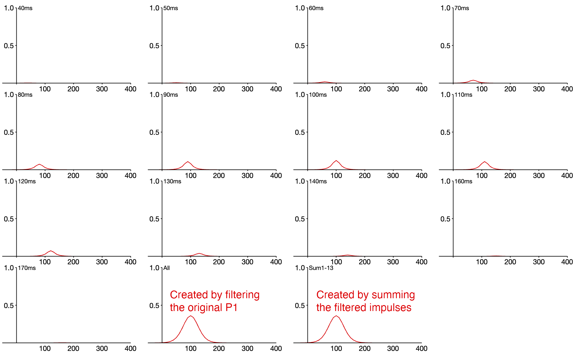
You should see something like Screenshot 4.19. Notice that each of the impulses in Channels 1–13 has been “smeared out” by the filter and looks like the filtered impulse response function that we saw in the preceding exercise. You can also see the filtered P1 wave in Channel 14.
Screenshot 4.19
Now we’re going to create a new Channel 15 that is the sum of the filtered impulses from Channels 1–13. To do this, go to the Channel Operations panel and type the following into the top row of the text box: ch15 = ch1+ch2+ch3+ch4+ch5+ch6+ch7+ch8+ch9+ch10+ch11+ch12+ch13 label Sum1-13. Once the panel is set up as shown in Screenshot 4.20, click Run.
Screenshot 4.20
As shown in Screenshot 4.21, you should now see that the new Channel 15, which was created by summing the filtered impulses in Channels 1-13, is exactly the same as Channel 14, which was created by filtering the P1 waveform as a whole.
Screenshot 4.21
This is analogous to what you saw in a previous exercise, where you filtered the individual P1, N1, and P2 waves and then summed them together, which created the same result as filtering the whole ERP waveform. Here, you filtered the impulses for each time point and then summed them together, which created the same result as filtering the whole P1 waveform.
Figure 4.5 puts all of this together. Panel E is a reminder of the impulse response function for the 10 Hz filter we have been using (i.e., the output of the filter when the input is a 1 µV impulse at time zero). Note that the peak amplitude is 0.14 µV.
Panel A shows that we can represent an ERP waveform as a set of impulses. [In this example, the sampling rate was 100 Hz, so there was one point every 10 ms. A sampling rate of 250 Hz (one point every 4 ms) would be more typical, but it’s easier to see the impulse responses at the slower rate.]
Figure 4.5. Overview of filtering in the time domain. (A) Unfiltered P1 waveform and corresponding impulses representing the voltage at each time point. (B) Filtered impulses for two of the impulses (indicated with blue and green impulses and waveforms). (C) All of the original and filtered impulses. (D) The filtered impulses along with the sum of the filtered impulses, which is equal to the filtered version of the P1 waveform. (E) Impulse response function of the 10 Hz filter used in this exercise and the preceding exercise.
Panel B shows the impulses, along with the filtered versions of two of the impulses (one shown in blue and the other shown in green). The filtered version of an impulse is essentially a copy of the filter’s impulse response function that has been shifted over to the time of the impulse and scaled by the height of the impulse. For example, the blue impulse in panel B leads to a copy of the impulse response function that is centered at the time of that impulse (70 ms) and is scaled by the height of the impulse (0.16 µV). The impulse response function was 0.24 µV at its peak, so the filtered version of the blue impulse has a peak height of 0.16 x 0.24 = 0.04 µV.
Panel C shows the filtered versions of all of the impulses. Each filtered version of an impulse is a copy of the impulse response function from Panel E that has been shifted so that it’s centered at the time of the impulse and scaled by the amplitude of the impulse.
Panel D shows that the filtered version of the P1 waveform can be created by summing together all of the filtered responses to the impulses (which are scaled-and-shifted copies of the impulse response function in Panel E). In other words, to filter a waveform, you replace each point in the waveform with a scaled-and-shifted copy of the impulse response function and then sum them together.
Congratulations—you now know how filtering works in the time domain! And I hope you can see how the shape of the filtered waveform is influenced by the shape of the impulse response function. For example, if we had a narrower impulse response function, the filtered waveform would be less “smeared out” than the one shown in Figure 4.5D.
I also played a little trick on you in this exercise: I taught you the mathematical concept of convolution without you realizing it. Convolution involves the same scaling-and-shifting process that is involved in filtering. When we convolve two functions, A and B, we replace each point in A with a scaled-and-shifted copy of B and then sum them together. That’s exactly what you just did when you filtered the P1 wave using the impulse response function of the 10 Hz filter: You filtered function A (the P1 waveform) by replacing each point in it with a scaled-and-shifted copy of function B (the impulse response function). In other words, filtering is achieved in the time domain by convolving the ERP waveform with the filter’s impulse response function. [See the box below for one additional detail about convolution.]
An additional detail about convolution
I left out one little detail about convolution in the discussion above. When we convolve functions A and B, we first mirror-reverse function B before we do the scaling-and-shifting process. However, if B is mirror-symmetrical, we don’t need to worry about this detail because the original and mirror-reversed versions of the function are identical. The software-based filters that we use for ERPs almost always have mirror-symmetrical impulse response functions, so the mirror-reversal step is unnecessary. This detail is only important for causal filters, which are used very rarely (see Chapter 8 in Luck, 2014, for more information).