Opening the book…
- Define precisely what it means for a limit to approach positive or negative infinity.
- Define the limit of a function as \(x\to +\infty\) or \(x\to -\infty\).
- Use graphs to approximate vertical and horizontal asymptotes.
- Use limits to find vertical and horizontal asymptotes of a given function.
So far, we stated that in the equation \( \lim\limits_{x\to c}f(x) = L\), both \(c\) and \(L\) were numbers. In this section we relax that definition a bit by considering situations when it makes sense to let \(c\) and/or \(L\) be "infinity.''
As a motivating example, consider \(f(x) = \dfrac{1}{x^2}\), as shown in Figure 1.30. Note how, as \(x\) approaches 0, \(f(x)\) grows very, very large. It seems appropriate, and descriptive, to state that
\[\lim_{x\rightarrow 0} \dfrac{1}{x^2}=\infty \nonumber \]
Also note that as \(x\) gets very large, \(f(x)\) gets very, very small. We could represent this concept with notation such as
\[\lim_{x\rightarrow \infty} \frac{1}{x^2}=0 \nonumber \]
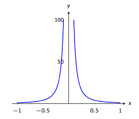
Figure \(\PageIndex{1}\): Graphing \(f(x)=\dfrac{1}{x^2}\) for values of \(x \text{ near }0\).
We explore both types of use of \(\infty\) in turn.
We say \( \lim\limits_{x\rightarrow c} f(x)=\infty\) if for every \(M>0\) there exists \(\delta>0\) such that for all \(x\neq c\), if \(|x-c|<\delta\), then \(f(x)\geq M\).
This is just like the \(\epsilon\)-\(\delta\) definition from Section 2.4. In that definition, given any (small) value \(\epsilon\), if we let \(x\) get close enough to \(c\) (within \(\delta\) units of \(c\)) then \(f(x)\) is guaranteed to be within \(\epsilon\) of \(f(c)\). Here, given any (large) value \(M\), if we let \(x\) get close enough to \(c\) (within \(\delta\) units of \(c\)), then \(f(x)\) will be at least as large as \(M\). In other words, if we get close enough to \(c\), then we can make \(f(x)\) as large as we want. We can define limits equal to \(-\infty\) in a similar way.
It is important to note that by saying \( \lim\limits_{x\to c}f(x) = \infty\) we are implicitly stating that the limit of \(f(x)\), as \(x\) approaches \(c\), does not exist. A limit only exists when \(f(x)\) approaches an actual numeric value. We use the concept of limits that approach infinity because it is helpful and descriptive.
Find \( \lim\limits_{x\rightarrow 1}\dfrac{1}{(x-1)^2}\) as shown in Figure \(\PageIndex{2}\).
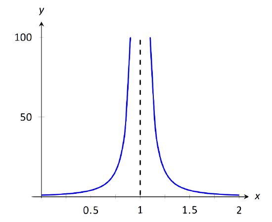
Figure \(\PageIndex{2}\): Observing infinite limit as \(x\to 1\) of \(\dfrac{1}{(x-1)^2}\)
Solution
Previously, by inspecting values of \(x\) close to 1 we concluded that this limit does not exist. That is, it cannot equal any real number. But the limit could be infinite. And in fact, we see that the function does appear to be growing larger and larger, as \(f(.99)=10^4\), \(f(.999)=10^6\), \(f(.9999)=10^8\).
A similar thing happens on the other side of 1. In general, let a "large'' value \(M\) be given. Let \(\delta=\dfrac{1}{\sqrt{M}}\).
If \(x\) is within \(\delta\) of 1, i.e., if \(|x-1|<\dfrac{1}{\sqrt{M}} \), then:
\[ |x-1| < \frac{1}{\sqrt{M}} \implies (x-1)^2 < \frac{1}{M} \implies \frac{1}{(x-1)^2} > M \nonumber \]
This is what we wanted to show, and we may now say \(\boxed{\lim\limits_{x\rightarrow 1}\dfrac{1}{(x-1)^2}=+\infty}\)
Find \(\lim\limits_{x\rightarrow 0}\dfrac{1}{x}\), as shown in Figure \(\PageIndex{3}\).
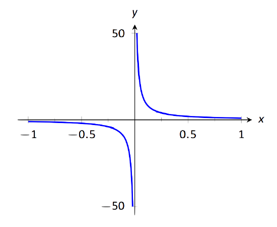
Figure \(\PageIndex{3}\): Observing infinite limit as \(x\to 0\) of \(\dfrac{1}{x}\)
Solution
It is easy to see that the function grows without bound near 0, but it does so in different ways on different sides of 0. Since its behavior is not consistent, we cannot say that \( \lim\limits_{x\to 0}\frac{1}{x}=+\infty\). However, we can make a statement about one--sided limits:
We can state that \( \lim\limits_{x\rightarrow 0^+}\dfrac1x=+\infty\) and \( \lim\limits_{x\rightarrow 0^-}\dfrac1x=-\infty\).
Since these do not match, we know \(\boxed{\lim_{x\to 0} \dfrac{1}{x}=\text{ DNE}}\)
Vertical Asymptotes
If the limit of \(f(x)\) as \(x\) approaches \(c\) from either the left or right (or both) is \(\infty\) or \(-\infty\), we say the function has a vertical asymptote at \(x=c\).
Find the vertical asymptotes of \(f(x)=\dfrac{3x}{x^2-4}\)
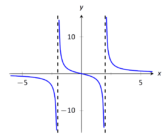
Figure \(\PageIndex{4}\): Graphing \(f(x) = \dfrac{3x}{x^2-4}\).
Solution
Vertical asymptotes occur where the function grows without bound; this can occur at values of \(c\) where the denominator is 0. When \(x\) is near \(c\), the denominator is small, which in turn can make the function take on large values. In the case of the given function, the denominator is 0 at \(x=\pm 2\). Substituting in values of \(x\) close to \(2\) and \(-2\) seems to indicate that the function tends toward \(\infty\) or \(-\infty\) at those points. We can graphically confirm this by looking at Figure \(\PageIndex{4}\). Thus the vertical asymptotes are at \(\boxed{x=2 \text{ and } x=-2}\)
Use limits to find the vertical asymptotes of \(f(x)=\dfrac{x^2-x-20}{x^2-16}\)
- Answer
-
Since \(\displaystyle \lim_{x\to 4^+}f(x)=-\infty\) and \(\displaystyle \lim_{x\to 4^-}f(x)=+\infty\), there is a vertical asymptote at \(x=4\).
Since \(\displaystyle \lim_{x\to -4^+}f(x)=\dfrac{9}{8}\) and \(\displaystyle \lim_{x\to -4^-}f(x)=\dfrac{9}{8}\), there is a hole instead at \(x=-4\), not a vertical asymptote.
When a rational function has a vertical asymptote at \(x=c\), we can conclude that the denominator is 0 at \(x=c\). However, just because the denominator is 0 at a certain point does not mean there is a vertical asymptote there. For instance, \(f(x)=\dfrac{x^2-1}{x-1}\) does not have a vertical asymptote at \(x=1\), as shown in Figure \(\PageIndex{5}\). While the denominator does get small near \(x=1\), the numerator gets small too, matching the denominator step for step. In fact, factoring the numerator, we get
\[f(x)=\dfrac{(x-1)(x+1)}{x-1} \nonumber \]
Canceling the common term, we get that \(f(x)=x+1\) for \(x\not=1\). So there is clearly no asymptote, rather a hole exists in the graph at \(x=1\).
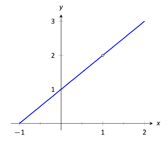
Figure \(\PageIndex{5}\): Graphically showing that \(f(x)=\dfrac{x^2-1}{x-1}\) does not have an asymptote at \(x=1\).
The above example may seem a little contrived. Another example demonstrating this important concept is \(f(x)=\dfrac{\sin (x)}{x}\). We have considered this function several times in the previous sections. We found that \( \lim\limits_{x\to0}\dfrac{\sin (x)}{x}=1\); i.e., there is no vertical asymptote. No simple algebraic cancellation makes this fact obvious; we instead use the Squeeze Theorem to prove this.
If the denominator is 0 at a certain point but the numerator is not, then there will usually be a vertical asymptote at that point. On the other hand, if the numerator and denominator are both zero at that point, then there may or may not be a vertical asymptote at that point. This case where the numerator and denominator are both zero returns us to an important topic.
Indeterminate Forms
We have seen how the limits
\[\lim\limits_{x\rightarrow 0}\frac{\sin x}{x}\quad \text{and}\quad \lim\limits_{x\to1}\frac{x^2-1}{x-1} \nonumber \]
each return the indeterminate form "\(\dfrac{0}{0}\)'' when we blindly plug in \(x=0\) and \(x=1\), respectively. However, \(\dfrac{0}{0}\) is not a valid arithmetical expression. It gives no indication that the respective limits are 1 and 2.
With a little cleverness, one can come up \(\dfrac{0}{0}\) expressions which have a limit of \(\infty\), 0, or any other real number. That is why this expression is called indeterminate.
A key concept to understand is that such limits do not really return \(\dfrac{0}{0}\). Rather, keep in mind that we are taking limits. What is really happening is that the numerator is shrinking to 0 while the denominator is also shrinking to 0. The respective rates at which they do this are very important and determine the actual value of the limit.
An indeterminate form indicates that one needs to do more work in order to compute the limit. That work may be algebraic (such as factoring and canceling) or it may require a tool such as the Squeeze Theorem. In a later section we will learn a technique called l'Hospital's Rule that provides another way to handle indeterminate forms.
Some other common indeterminate forms are \(\infty-\infty\), \(\infty\cdot 0\), \(\dfrac{\infty}{\infty}\), \(0^0\), \(\infty^0\) and \(1^{\infty}\). Again, keep in mind that these are the "blind'' results of evaluating a limit, and each, in and of itself, has no meaning. The expression \(\infty-\infty\) does not really mean "subtract infinity from infinity.'' Rather, it means "One quantity is subtracted from the other, but both are growing without bound.'' What is the result? It is possible to get every value between \(-\infty\) and \(\infty\)
Note that \(\dfrac{1}{0}\) and \(\dfrac{\infty}{0}\) are not indeterminate forms, though they are not exactly valid mathematical expressions, either. In each, the function is growing without bound, indicating that the limit will be \(\infty\), \(-\infty\), or simply not exist if the left- and right-hand limits do not match.
Limits at Infinity and Horizontal Asymptotes
At the beginning of this section we briefly considered what happens to \(f(x) = \dfrac{1}{x^2}\) as \(x\) grew very large. Graphically, it concerns the behavior of the function to the "far right'' of the graph. We make this notion more explicit in the following definition.
- We say \(\lim\limits_{x\rightarrow\infty} f(x)=L\) if for every \(\epsilon>0\) there exists \(M>0\) such that if \(x\geq M\), then \(|f(x)-L|<\epsilon\).
- We say \(\lim\limits_{x\rightarrow-\infty} f(x)=L\) if for every \(\epsilon>0\) there exists \(M<0\) such that if \(x\leq M\), then \(|f(x)-L|<\epsilon\).
- If \(\lim\limits_{x\rightarrow\infty} f(x)=L\) or \(\lim\limits_{x\rightarrow-\infty} f(x)=L\), we say that \(y=L\) is a horizontal asymptote of \(f\).
We can also define limits such as \(\lim\limits_{x\rightarrow\infty}f(x)=\infty\) by combining this definition with Definition 5.
Approximate the horizontal asymptote(s) of \( f(x)=\dfrac{x^2}{x^2+4}\)
Solution
We will approximate the horizontal asymptotes by approximating the limits
\[\lim\limits_{x\to-\infty} \frac{x^2}{x^2+4}\quad \text{and}\quad \lim\limits_{x\to\infty} \frac{x^2}{x^2+4} \nonumber \]
Figure \(\PageIndex{6}\) shows a sketch of \(f\), and part (b) gives values of \(f(x)\) for large magnitude values of \(x\). It seems reasonable to conclude from both of these sources that \(f\) has a horizontal asymptote at \(\boxed{y=1}\)
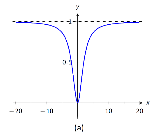
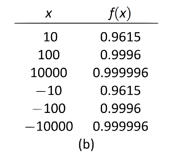
Figure \(\PageIndex{6}\): Using a graph and a table to approximate a horizontal asymptote of \( f(x)=\dfrac{x^2}{x^2+4}\)
Soon, we will show how to determine this analytically.
Horizontal asymptotes can take on a variety of forms. Figure \(\PageIndex{7(a)}\) shows that \(f(x) = \dfrac{x}{x^2+1}\) has a horizontal asymptote of \(y=0\), where 0 is approached from both above and below.
Figure \(\PageIndex{7(b)}\) shows that \(f(x) =\dfrac{x}{\sqrt{x^2+1}}\) has two horizontal asymptotes; one at \(y=1\) and the other at \(y=-1\).
Figure \(\PageIndex{7(c)}\) shows that \(f(x) = \dfrac{\sin (x)}{x}\) has even more interesting behavior than at just \(x=0\); as \(x\) approaches \(\pm\infty\), \(f(x)\) approaches 0, but oscillates as it does this.
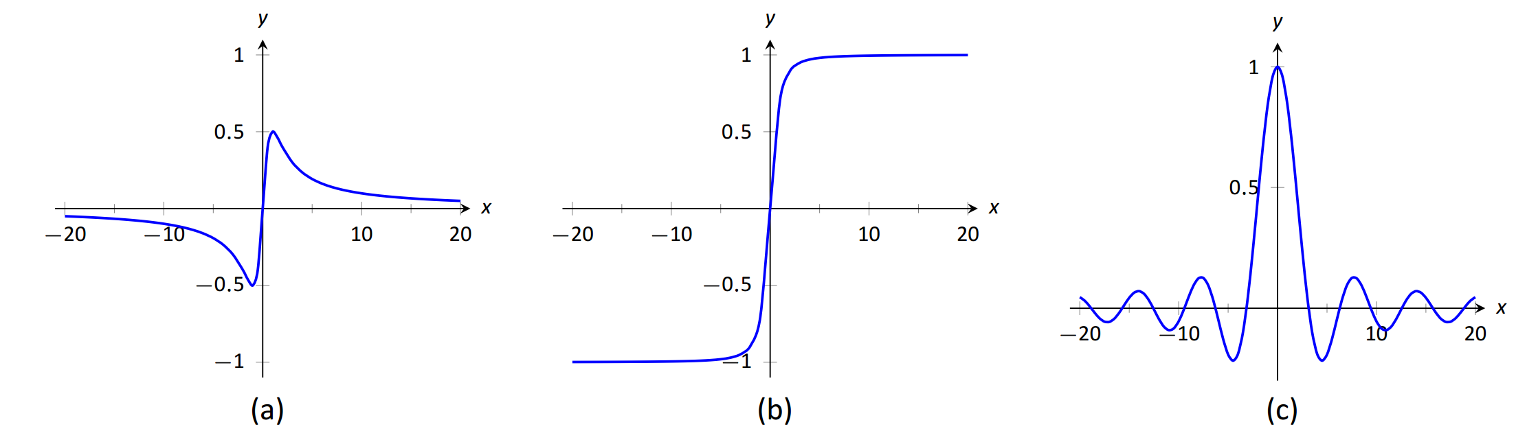
Figure \(\PageIndex{7}\): Considering different types of horizontal asymptotes.
We can analytically evaluate limits at infinity for rational functions once we understand \(\lim\limits_{x\rightarrow\infty} \dfrac{1}{x}\). As \(x\) gets larger and larger, the \(\dfrac{1}{x}\) gets smaller and smaller, approaching 0. We can, in fact, make \(\dfrac{1}{x}\) as small as we want by choosing a large enough value of \(x\). Given \(\epsilon\), we can make \(\dfrac{1}{x}<\epsilon\) by choosing \(x>\dfrac{1}{\epsilon}\). Thus we have \(\lim\limits_{x\rightarrow\infty} \dfrac{1}{x}=0\).
It is now not much of a jump to conclude the following two results will hold for any \(n>0\):
\[\lim\limits_{x\rightarrow\infty}x^{-n}=0\quad \text{and}\quad \lim\limits_{x\rightarrow-\infty}x^{-n}=0 \nonumber \]
Now suppose we need to compute the following limit:
\[\lim\limits_{x\rightarrow\infty}\frac{x^3+2x+1}{4x^3-2x^2+9} \nonumber\]
A good way of approaching this is to divide through the numerator and denominator by \(x^3\) (hence dividing by 1), which is the largest power of \(x\) to appear in the function. Doing this, we get
\[\lim\limits_{x\rightarrow\infty}\frac{x^3+2x+1}{4x^3-2x^2+9} =\lim\limits_{x\rightarrow\infty}\dfrac{x^{-3}}{x^{-3}}\cdot\dfrac{x^3+2x+1}{4x^3-2x^2+9}=\lim\limits_{x\rightarrow\infty}\frac{1+2x^{-2}+x^{-3}}{4-2x^{-1}+9x^{-3}} =\dfrac{1+0+0}{4-0+0}=\dfrac{1}{4} \nonumber \]
This procedure works for any rational function. In fact, it gives us the following theorem.
Let \(f(x)\) be a rational function of the following form:
\[f(x)=\frac{a_nx^n + a_{n-1}x^{n-1}+\dots + a_1x + a_0}{b_mx^m + b_{m-1}x^{m-1} + \dots + b_1x + b_0} \nonumber \]
where any of the coefficients may be 0 except for \(a_n\) and \(b_m\).
- If \(n=m\), then \(\lim\limits_{x\rightarrow\infty} f(x) = \lim\limits_{x\rightarrow-\infty} f(x) = \dfrac{a_n}{b_m}\).
- If \(n<m\), then \(\lim\limits_{x\rightarrow\infty} f(x) = \lim\limits_{x\rightarrow-\infty} f(x) = 0\).
- If \(n>m\), then \(\lim\limits_{x\rightarrow\infty} f(x)\) and \(\lim\limits_{x\rightarrow-\infty} f(x)\) are both infinite.
We can see why this is true:
If the highest power of \(x\) is the same in both the numerator and denominator (i.e. \(n=m\)), we will be in a situation like the example above, where we will divide by \(x^n\) and in the limit all the terms will approach 0 except for \(a_n\) and \(b_m\). Since \(n=m\), this will leave us with the limit \(\dfrac{a_n}{b_m}\).
If \(n<m\), then after dividing through by \(x^m\), all the terms in the numerator will approach 0 in the limit, leaving us with \(\dfrac{0}{b_m}\) or 0.
If \(n>m\), and we try dividing through by \(x^n\), we end up with all the terms in the denominator tending toward 0, while the \(x^n\) term in the numerator does not approach 0. This is indicative of some sort of infinite limit.
Intuitively, as \(x\) gets very large, all the terms in the numerator are small in comparison to \(a_nx^n\), and likewise all the terms in the denominator are small compared to \(b_mx^m\). If \(n=m\), looking only at these two important terms, we have \(\dfrac{a_nx^n}{b_nx^m}\), which reduces to \(\dfrac{a_n}{b_m}\). If \(n<m\), the function behaves like \(\dfrac{a_n}{b_mx^{m-n}}\), which tends toward 0. If \(n>m\), the function behaves like \(\dfrac{a_nx^{n-m}}{b_m}\), which will tend to either \(\infty\) or \(-\infty\) depending on the values of \(n\), \(m\), \(a_n\), \(b_m\) and whether you are looking for \(\lim\limits_{x\rightarrow\infty} f(x)\) or \(\lim\limits_{x\rightarrow-\infty} f(x)\).
With care, we can quickly evaluate limits at infinity for a large number of functions by considering the largest powers of \(x\). For instance, consider again \(\lim\limits_{x\to\pm\infty}\dfrac{x}{\sqrt{x^2+1}},\) graphed in Figure \(\PageIndex{7(b)}\). When \(x\) is very large, \(x^2+1 \approx x^2\). Thus
\[\sqrt{x^2+1}\approx \sqrt{x^2} = |x|\quad \text{and}\quad \frac{x}{\sqrt{x^2+1}} \approx \frac{x}{|x|} \nonumber \]
This expression is 1 when \(x\) is positive and \(-1\) when \(x\) is negative. Hence we get asymptotes of \(y=1\) and \(y=-1\), respectively.
We will confirm analytically that \(y=1\) is the horizontal asymptote of \( f(x) = \dfrac{x^2}{x^2+4}\), as approximated in Example \(\PageIndex{4}\).
Before using Theorem \(\PageIndex{1}\), let's use the technique of evaluating limits at infinity of rational functions that led to that theorem. The largest power of \(x\) in \(f\) is 2, so divide the numerator and denominator of \(f\) by \(x^2\), then take limits.
\[\lim\limits_{x\to\infty}\frac{x^2}{x^2+4} = \lim\limits_{x\to\infty}\frac{x^{-2}}{x^{-2}}\cdot \dfrac{x^2}{x^2+4}=\lim_{x\to \infty} \dfrac{1}{1+4x^{-2}}=\dfrac{1}{1+0}= 1 \nonumber \]
We can also use Theorem \(\PageIndex{1}\) directly; in this case \(n=m\) so the limit is the ratio of the leading coefficients of the numerator and denominator, i.e., \(\dfrac{1}{1}=1\). Therefore, we know \(f(x)\) has a horizontal asymptote at \(y=1\).
Use Theorem \(\PageIndex{1}\) to evaluate each of the following limits.
(a) \(\displaystyle \lim\limits_{x\rightarrow-\infty}\dfrac{x^2+2x-1}{x^3+1} \)
(b) \(\displaystyle \lim\limits_{x\rightarrow\infty}\frac{x^2+2x-1}{1-x-3x^2}\)
(c) \(\displaystyle \lim\limits_{x\rightarrow\infty}\frac{x^2-1}{3-x} \)
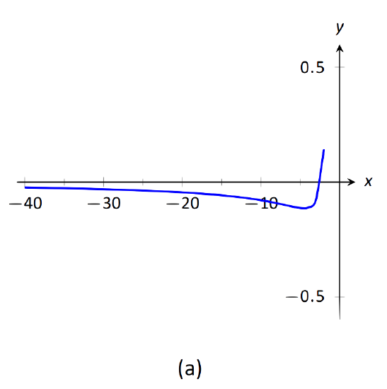
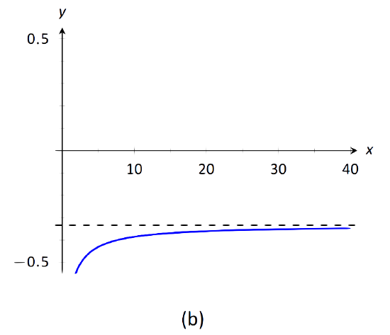
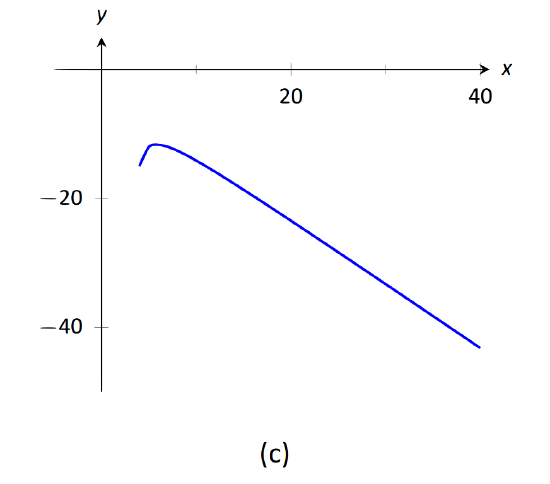
Figure \(\PageIndex{8}\): Visualizing the functions in Example \(\PageIndex{6}\).
Solution
(a) The highest power of \(x\) is in the denominator. Therefore, the limit is \(\boxed{0}\)
(b) The highest power of \(x\) is \(x^2\), which occurs in both the numerator and denominator. The limit is therefore the ratio of the coefficients of \(x^2\), which is \(\boxed{-\dfrac{1}{3}}\)
(c) The highest power of \(x\) is in the numerator so the limit will be \(\infty\) or \(-\infty\). To see which, consider only the dominant terms from the numerator and denominator, which are \(x^2\) and \(-x\). The expression in the limit will behave like \(\dfrac{x^2}{-x} = -x\) for large values of \(x\). Therefore, the limit is \(\boxed{-\infty}\)
Evaluate the following limits.
(a) \(\displaystyle \lim_{x\to \infty} \dfrac{\sqrt{4x^2+1}}{4x+3}\)
(b) \(\displaystyle \lim_{x\to -\infty} \dfrac{\sqrt{4x^2+1}}{4x+3}\)
- Answer (a)
-
For large positive \(x\), we know \(\sqrt{4x^2+1}\approx \sqrt{4x^2}=|2x|=2x\),
so the limit becomes \(\displaystyle{ \lim_{x\to \infty} \dfrac{2x}{4x}=\dfrac{1}{2}}\)
- Answer (b)
-
For large negative \(x\), we know \(\sqrt{4x^2+1}\approx \sqrt{4x^2}=|2x|=-2x\),
so the limit becomes \(\displaystyle{ \lim_{x\to \infty} \dfrac{-2x}{4x}=-\dfrac{1}{2}}\)
Key Concepts
- A limit approaches positive (or negative) infinity if \(f(x)\) grows arbitrarily large (or arbitrarily large and negative) as \(x\to a\).
- A limit as \(x\to +\infty\) (or \(x\to -\infty\)) describes what \(f(x)\) approaches as \(x\) grows arbitrarily large (or arbitrarily large and negative)
- Vertical Asymptotes occur at \(x=c\) whenever \(\displaystyle{\lim_{x\to c^+}f(x)=\pm \infty}\) or \(\displaystyle{\lim_{x\to c^-}f(x)=\pm \infty}\).
- Horizontal Asymptotes occur at \(y=L\) whenever \(\displaystyle{\lim_{x\to +\infty}f(x)=L}\) or \(\displaystyle{\lim_{x\to +\infty}f(x)=L}\).
Why? Mathematics is famous for building on itself and calculus proves to be no exception. In the next chapter we will be interested in "dividing by 0.'' That is, we will want to
These are just two quick examples of why we are interested in limits. Many students dislike this topic when they are first introduced to it, but over time an appreciation is often formed based on the scope of its applicability.
Glossary
- indeterminant form
- A limit of a function is an indeterminant form if it results in an attempt to evaluate \(\dfrac{0}{0}, \dfrac{\infty}{\infty}, \infty\cdot 0, \infty -\infty, 1^\infty\), or \(\infty^0\).
- horizontal asmptote
- A function has a horizontal asymptote \(y=L\) whenever \(\displaystyle{\lim_{x\to +\infty}f(x)=L}\) or \(\displaystyle{\lim_{x\to +\infty}f(x)=L}\).
- vertical asymptote
- A function has a vertical asymptote \(x=c\) whenever \(\displaystyle{\lim_{x\to c^+}f(x)=\pm \infty}\) or \(\displaystyle{\lim_{x\to c^-}f(x)=\pm \infty}\).
This page titled 2.6: Limits at Infinity; Horizontal Asymptotes was last modified on Sun, 12 Apr 2026 14:16:42 GMT and is shared under a CC BY-NC-SA 4.0 license and was authored, remixed, and/or curated by Leonard Lamp, Kenn Huber, and Mohamad Youssef.
The book could not be loaded just now.