Opening the book…
Stokes’ Theorem says we can calculate the flux of \( \text{curl} (\vecs{F})\) across surface \(S\) by knowing information only about the values of \(\vecs{F}\) along the boundary of \(S\). Conversely, we can calculate the line integral of vector field \(\vecs{F}\) along the boundary of surface \(S\) by translating to a double integral of the curl of \(\vecs{F}\) over \(S\).
Let \(S\) be a smooth, oriented surface with unit normal vector \(\vecs{N}\). Suppose the boundary of \(S\) is a simple closed curve \(C\). The orientation of \(S\) induces the positive orientation of \(C\) if, when traversing \(C\) with your head pointing in the direction of \(\vecs{N}\), the surface is always on your left. With this definition in place, we can state Stokes’ Theorem.
Let \(S\) be a piecewise smooth oriented surface with a boundary that is a simple closed curve \(C\) with positive orientation. If \(\vecs{F}\) is a vector field with component functions that have continuous partial derivatives on an open region containing \(S\), then
\[\int_C \vecs{F} \cdot d \vecs{r} = \iint_S \text{curl} ( \vecs{F} )\cdot d\vecs S \nonumber \]
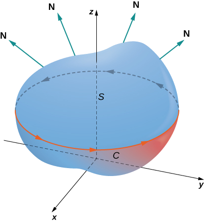
We saw in the previous section that Green’s Theorem is a special case of Stokes’ Theorem. Green’s Theorem can only handle surfaces in a plane, but Stokes’ Theorem can handle surfaces in a plane or in space.
The complete proof of Stokes’ Theorem is beyond the scope of this text. We look at an intuitive explanation for the truth of the theorem and then see proof of the theorem in the special case that surface \(S\) is a portion of a graph of a function, and \(S\), the boundary of \(S\), and \(\vecs{F}\) are all fairly tame.
First, we look at an informal proof of the theorem. This proof is not rigorous, but it is meant to give a general feeling for why the theorem is true. Let \(S\) be a surface and let \(D\) be a small piece of the surface so that \(D\) does not share any points with the boundary of \(S\). We choose \(D\) to be small enough so that it can be approximated by an oriented square \(E\). Let \(D\) inherit its orientation from \(S\), and give \(E\) the same orientation. This square has four sides; denote them \(E_l, \, E_r, \, E_u\), and \(E_d\) for the left, right, up, and down sides, respectively. On the square, we can use the flux form of Green’s theorem:
\[\int_{E_l+E_d+E_r+E_u} \vecs{F} \cdot d \vecs{r} = \iint_E \text{curl} ( \vecs{F}) \cdot \vecs{N} \, dS = \iint_E \text{curl}( \vecs{F}) \cdot d\vecs{S} \nonumber \]
To approximate the flux over the entire surface, we add the values of the flux on the small squares approximating small pieces of the surface.
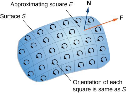
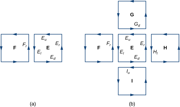
By Green’s theorem, the flux across each approximating square is a line integral over its boundary. Let \(F\) be an approximating square with an orientation inherited from \(S\) and with a right side \(E_l\) (so \(F\) is to the left of \(E\)). Let \(F_r\) denote the right side of \(F\); then, \(E_l = - F_r\). In other words, the right side of \(F\) is the same curve as the left side of \(E\), just oriented in the opposite direction. Therefore,
\[\int_{E_l} \vecs F \cdot d\vecs r = - \int_{F_r} \vecs F \cdot d\vecs r \nonumber \]
As we add up all the fluxes over all the squares approximating surface \(S\), line integrals
\[\int_{E_l} \vecs{F} \cdot d \vecs{r} \quad \text{ and } \quad \int_{F_r} \vecs{F} \cdot d\vecs{r} \nonumber \]
cancel each other out. The same goes for the line integrals over the other three sides of \(E\). These three line integrals cancel out with the line integral of the lower side of the square above \(E\), the line integral over the left side of the square to the right of \(E\), and the line integral over the upper side of the square below \(E\). After all this cancelation occurs over all the approximating squares, the only line integrals that survive are the line integrals over sides approximating the boundary of \(S\). Therefore, the sum of all the fluxes (which, by Green’s theorem, is the sum of all the line integrals around the boundaries of approximating squares) can be approximated by a line integral over the boundary of \(S\). In the limit, as the areas of the approximating squares go to zero, this approximation gets arbitrarily close to the flux.
Let’s now look at a rigorous proof of the theorem in the special case that \(S\) is the graph of function \(z = f(x,y)\), where \(x\) and \(y\) vary over a bounded, simply connected region \(D\) of finite area. Furthermore, assume that \(f\) has continuous second-order partial derivatives. Let \(C\) denote the boundary of \(S\) and let \(C'\) denote the boundary of \(D\). Then, \(D\) is the “shadow” of \(S\) in the plane and \(C'\) is the “shadow” of \(C\) as shown below. Suppose that \(S\) is oriented upward. The counterclockwise orientation of \(C\) is positive, as is the counterclockwise orientation of \(C'\). Let \(\vecs F(x,y,z) = \langle P,Q,R \rangle\) be a vector field with component functions that have continuous partial derivatives.
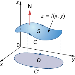
We take the standard parameterization of \(S \): \(\vecs{r}(u,v)=\langle u, v,f(u,v)\rangle \).
The tangent vectors are \(\vecs r_u = \langle 1,0,f_x(u,v) \rangle\) and \(\vecs r_v = \langle 0,1,f_y(u,v) \rangle\), and therefore, \(\vecs r_u \times \vecs r_v = \langle -f_x(u,v), \, -f_y(u,v), \, 1 \rangle\).
\[\iint_S \text{curl} ( \vecs{F}) \cdot d\vecs{S} = \iint_D [- (R_y - Q_z)z_x - (P_z - R_x)z_y + (Q_x - P_y)] \, dA \nonumber \]
where the partial derivatives are all evaluated at \((u,v,f(u,v))\), making the integrand depend on \(x\) and \(y\) only. Suppose \(\langle x (t), \, y(t) \rangle, \, a \leq t \leq b\) is a parameterization of \(C'\). Then, a parameterization of \(C\) is \(\langle x (t), \, y(t), \, f(x(t), \, y(t))\rangle, \, a \leq t \leq b\). Armed with these parameterizations, the Chain rule, and Green’s Theorem, and keeping in mind that \(P\), \(Q\) and \(R\) are all functions of \(x\) and \(y\), we can evaluate line integral
\[ \begin{align*} \int_C \vecs{F} \cdot d \vecs{r} &= \int_a^b (Px'(t) + Qy'(t) + Rz'(t)) \, dt \\[4pt] &= \int_a^b \left[Px'(t) + Qy'(t) + R\left(\dfrac{\partial z}{\partial x} \dfrac{dx}{dt} + \dfrac{\partial z}{\partial y} \dfrac{dy}{dt}\right) \right] dt \\[4pt] &= \int_a^b \left[ \left(P + R \dfrac{\partial z}{\partial x} \right) x' (t) + \left(Q + R \dfrac{\partial z}{\partial y} \right) y'(t) \right] dt \\[4pt] &= \int_{C'} \left(P + R \dfrac{\partial z}{\partial x} \right)\, dx + \left(Q + R \dfrac{\partial z}{\partial y} \right) \, dy \\[4pt] &= \iint_D \left[ \dfrac{\partial}{\partial x} \left( Q + R \dfrac{\partial z}{\partial y} \right) - \dfrac{\partial}{\partial y} \left(P + R \dfrac{\partial z}{\partial x} \right) \right] \, dA \\[4pt] &=\iint_D \left(\dfrac{\partial Q}{\partial x} + \dfrac{\partial Q}{\partial z} \dfrac{\partial z}{\partial x} + \dfrac{\partial R}{\partial x} \dfrac{\partial z}{\partial y} + \dfrac{\partial R}{\partial z}\dfrac{\partial z}{\partial x} \dfrac{\partial z}{\partial y} + R \dfrac{\partial^2 z}{\partial x \partial y} \right) - \left(\dfrac{\partial P}{\partial y} + \dfrac{\partial P}{\partial z} \dfrac{\partial z}{\partial y} + \dfrac{\partial R}{\partial z} \dfrac{\partial z}{\partial y} \dfrac{\partial z}{\partial x} + R \dfrac{\partial^2 z}{\partial y \partial x} \right) \end{align*} \nonumber \]
By Clairaut’s Theorem, \(\dfrac{\partial^2 z}{\partial x \partial y} = \dfrac{\partial^2 z}{\partial y \partial x} \).
Therefore, four of the terms disappear from this double integral, and we are left with
\[\iint_D [- (R_y - Q_z)z_x - (P_z - R_x) z_y + (Q_x - P_y)] \, dA, \nonumber \]
which equals
\[\iint_S \text{curl} (\vecs{F} )\cdot d\vecs{S}\nonumber \]
We have shown that Stokes’ Theorem is true in the case of a function with a domain that is a simply connected region of finite area. We can quickly confirm this theorem for another important case: when vector field \(\vecs{F}\) is a conservative field. If \(\vecs{F}=\nabla f\) is conservative, the curl of \(\vecs{F}\) is zero, so
\[\iint_S \text{curl} ( \vecs{F}) \cdot d\vecs{S} = 0 \nonumber \]
Since the boundary of \(S\) is a closed curve, we know any parameterization of it \(\vecs{r}(t)\) for \(a\le t\le b\) will have \(\vecs{r}(a)=\vecs{r}(b)\). Therefore, the integral
\[\int_C \vecs{F} \cdot d\vecs{r}=f\left(\vecs{r}(b)\right)-f\left(\vecs{r}(a)\right) =0 \nonumber \]
Once again, these match, and Stokes' Theorem holds.
We will verify that Stokes’ Theorem is true for vector field \(\vecs{F}(x,y) = \langle -z,x,0 \rangle\) and surface \(S\), where \(S\) is the hemisphere, oriented outward, with parameterization \(\vecs r(u, v) = \langle \sin (u)\cos(v) , \sin(u) \sin(v), \cos(u) \rangle\) over \(D=\left\{ (u,v) \, : \, 0\le u\le \pi, \, 0\le v\le \pi \right\}\)
Let \(C\) be the boundary of \(S\). Note that \(C\) is a circle of radius 1, centered at the origin, sitting in plane \(y = 0\).

We want it to look counterclockwise when viewed from the positive \(y\)-axis (where the surface orientation is pointing), so we use the parameterization \(\vecs{r}(t)=\langle \sin(t), 0, \cos(t) \rangle\) for \( 0 \leq t \leq 2\pi\). Thus the line integral on \(C\) is:
\[ \begin{align*} \int_C \vecs{F} \cdot d \vecs{r} &= \int_0^{2\pi} \langle -\cos(t), \sin(t),0 \rangle \cdot \langle \cos(t), 0 , -\sin (t) \rangle \, dt \\[4pt] &= \int_0^{2\pi} -\cos^2(t) \, dt \\[4pt] &= \int_0^{2\pi} -\dfrac{1}{2}-\dfrac{1}{2}\cos (2t) \, dt \\[4pt] &= \left[ -\dfrac{1}{2}t - \dfrac{1}{4}\sin(2t) \right]\Bigg|_0^{2\pi} \\[4pt] & = -\pi \end{align*}\]
We know that \(\vecs{r}_u=\langle \cos(u) \cos(v), \cos(u) \sin(v) , -\sin(u)\rangle\) and \(\vecs{r}_v=\langle -\sin(u) \sin(v), \sin(u) \cos(v), 0\rangle\).
Therefore, \(\vecs{r}_u\times \vecs{r}_v = \langle \sin^2(u) \cos(v), \sin^2(u)\sin(v), \sin(u)\cos(u) \rangle \)
This points outward, so we have positive orientation in our surface integral.
We easily calculate that \(\text{curl}(\vecs{F})=\langle 0, -1,1 \rangle\). The flux of this over \(S\) is:
\[ \begin{align*} \iint_S \, \text{curl} (\vecs{F}) \cdot d\vecs S &= \iint_D \langle 0, -1, 1 \rangle \cdot \langle \sin^2(u)\cos(v), \sin^2(u)\sin(v), \sin(u)\cos(u) \rangle \, dA \\[4pt] &= \int_0^{\pi} \int_0^{\pi} (\sin(u)\cos(u)-\sin^2(u)\sin(v)) \, du \,dv \\[4pt] &= \int_0^{\pi} \left[ v\sin(u)\cos(u)+\sin^2(u)\cos(v) \right]\Big|_0^\pi \, du \\[4pt] &= \int_0^{\pi} (\pi \sin(u)\cos(u)-2\sin^2(u)) \, du \\[4pt] &= \int_0^{\pi} (\pi \sin(u)\cos(u)-1+\cos(2u)) \, du \\[4pt] &= \left[ \dfrac{\pi}{2}\sin^2(u)-u+\dfrac{1}{2}\sin(2u)\right]\Bigg|_0^\pi \\[4pt] &= -\pi \end{align*}\]
We have verified Stokes’ Theorem for this example.
We will calculate the line integral
\[\int_C \vecs{F} \cdot d\vecs{r} \nonumber \]
where \(\vecs{F} = \langle xy, \, x^2 + y^2 + z^2, \, yz \rangle\) and \(C\) is the boundary of the parallelogram with vertices \((0,0,1), \, (0,1,0), \, (2,0,-1)\), and \((2,1,-2)\)
To calculate the line integral directly, we need to parameterize each side of the parallelogram separately, calculate four separate line integrals, and add the results. This is not overly complicated, but it is time-consuming.

By contrast, let’s calculate the line integral using Stokes’ Theorem. Let \(S\) denote the surface of the parallelogram.
We can see the parallelogram has adjacent sides determined by the vectors \(\vecs{a}=\langle 0,1,-1\rangle\) and \(\vecs{b}=\langle 2,0,-2\rangle\). The normal vector to the plane containing this parallelogram must therefore be \(\vecs{n}=\vecs{a}\times \vecs{b}= \langle -2,-2,-2\rangle \). Plugging in any of our four vertices and simplifying gives the plane as \(x+y+z=1\).
Therefore, \(S\) is the portion of the graph of \(z = 1 - x - y\) for \((x,y)\) varying over the rectangular region with vertices \((0,0), \, (0,1), \, (2,0)\), and \((2,1)\) in the \(xy\)-plane. Therefore, a parameterization of \(S\) is \(\vecs{r}(u,v)=\langle u,v, \, 1 - u - v \rangle\) with \(0 \leq u \leq 2, \, 0 \leq v \leq 1\).
\[ \vecs{r}_u=\langle 1,0,-1\rangle, \quad \vecs{r}_v=\langle 0,1,-1\rangle, \quad \text{ and} \quad \vecs{r}_u\times \vecs{r}_v=\langle 1, 1, 1 \rangle \nonumber \]
Finally, the curl of \(\vecs{F}\) is easily calculated to be \( \langle -z, \, 0, \, x \rangle\), so by Stokes’ Theorem:
\[ \begin{align*} \int_C \vecs{F} \cdot d\vecs{r} &= \iint_S \text{curl}( \vecs{F}) \cdot d\vecs{S} \\[4pt] &= \int_0^2 \int_0^1 \langle -(1-u-v),0,u \rangle \cdot \langle 1, 1, 1\rangle \, dv \, du \\[4pt] &= \int_0^2 \int_0^1 (2u + v - 1) \, dv \, du \\[4pt] &= \int_0^2 \left[ 2uv + \dfrac{1}{2}v^2 - v\right]\Bigg|_0^1 \, du \\[4pt] &= \int_0^2 \left( 2u - \dfrac{1}{2}\right) \, du \\[4pt] &= \left[ u^2 - \dfrac{1}{2}u\right]\Bigg|_0^2 \\[4pt] & = 3\end{align*} \nonumber \]
Just like in Green's Theorem, if the curve of a line integral in \(\mathbb{R}^3\) is not closed, we can close it in order to use Stokes' Theorem.
If \(C\) is the curve defined by the straight lines \(\vecs{r}(t)=\left\langle t, t, t^2\right\rangle\) for \(-1\le t\le 1\), we evaluate the line integral
\[ \int_C y \, dx - xy \, dy + z^z \, dz \nonumber\]
This line integral is not pleasant to solve directly, and also is not closed so we cannot immediately use Stokes' Theorem. Instead we look to add another curve to it (that we can evaluate the line integral of) to close it, and then use Stokes' Theorem on them together.

We define \(C_1\) to be the curve connecting these endpoints. It is best to use the straight line with a constant \(z\) value to simplify the new line integral. So this can be parameterized by \(\vecs{s}(t)=\langle -t, -t, 1\rangle\) for \(-1 \le t\le 1 \)
For the vector field \(\vecs{F}=\langle y,-xy,z^z \rangle\) we can evaluate:
\[ \int_{C_1} \vecs{F}\cdot d\vecs{r} = \int_{-1}^{1} \left\langle -t,-t^2, 1^1 \right\rangle \cdot \langle -1,-1, 0 \rangle \, dt= \int_{-1}^1 t^2+t \, dt = \left[ \dfrac{1}{3} t^3+\dfrac{1}{2}t^2 \right] \Bigg|_{-1}^{1}= \dfrac{2}{3} \nonumber \]
Now since \(C\cup C_1\) is closed, we can consider any surface \(S\) with boundary \(C\cup C_1\) to use Stokes' Theorem on.
One such surface is the plane \(x=y\) on which these curves all lie. This is parameterized by \(\vecs{r}(u,v)=\langle u,u, v \rangle \) over \(D=\left\{ (u,v)\, : \, -1\le u\le 1, \, u^2 \le v\le 1 \right\}\)
\[ \vecs{r}_u=\langle 1,1,0 \rangle, \quad \vecs{r}_v=\langle 0,0,1 \rangle, \quad \text{ and } \quad \vecs{r}_u\times \vecs{r}_v=\langle 1, -1, 0 \rangle \nonumber \]
This points forward in the picture above, which matches the orientation of the boundary curve \(C\cup C_1\)
We calculate \(\text{curl}(\vecs{F})=\left\langle 0,0,-1-y \right\rangle\) and now can find the flux on \(S\):
\[ \iint_{S} \text{curl}(\vecs{F})\cdot d\vecs{S} = \iint_D \left\langle -0,0, -1-u\right\rangle \cdot \langle 1,-1,0 \rangle \, dA = \iint_D 0 \, dA = 0 \nonumber \]
Now we put these together using Stokes' Theorem:
\[ \iint_{S} \text{curl}(\vecs{F})\cdot d\vecs{S} = \int_{C} \vecs{F}\cdot d\vecs{r}+ \int_{C_1} \vecs{F}\cdot d\vecs{r} \nonumber \]
Therefore:
\[ \int_{C} \vecs{F}\cdot d\vecs{r}= \iint_{S} \text{curl}(\vecs{F})\cdot d\vecs{S} - \int_{C_1} \vecs{F}\cdot d\vecs{r} = 0-\dfrac{2}{3}=-\dfrac{2}{3} \nonumber\]
This page titled 4.3: Stokes’ Theorem was last modified on Tue, 12 May 2026 23:01:40 GMT and is shared under a CC BY-NC 4.0 license and was authored, remixed, and/or curated by Kenn Huber via source content that was edited to the style and standards of the LibreTexts platform.
The book could not be loaded just now.
Stokes’ Theorem translates between the flux integral of surface \(S\) to a line integral around the boundary of \(S\). Therefore, the theorem allows us to compute surface integrals or line integrals that would ordinarily be quite difficult by translating the line integral into a surface integral or vice versa. We now study some examples of each kind of translation.
Example \(\PageIndex{1}\): Calculating a Surface Integral
Let \(S\) be the surface defined by \(\vecs{r}(u,v)=\left\langle (v^2+v\cos(u))\cos(\pi v), (v^2+v\cos(u))\sin(\pi v), v^2+v\sin(u)\right\rangle\) for \(0\le u\le 2\pi\) and \(0\le v\le 2\), oriented outward.
If \(\vecs{F} = \langle x-z, e^{xz}, y^3+x \rangle\), calculate surface integral
\[\iint_S \text{curl} ( \vecs{F}) \cdot d\vecs S \nonumber \]
Solution
Note that to calculate \( \displaystyle \iint_S \text{curl} ( \vecs{F}) \cdot d\vecs S \) without using Stokes’ Theorem, we would need to find \(\vecs{r}_u, \vecs{r}_v\) and \(\vecs{r}_u\times \vecs{r}_v\), as well as the curl of \(\vecs{F}\).
Instead of doing all of that work, we use Stokes’ Theorem, noting that the boundary \(C\) of the surface is merely a single circle at \(v=2\). Replacing \(u\) with \(t\) gives us its parameterization:
\[ \vecs{r}(t)=\langle 4+2\cos(t), 0, 4+2\sin(t)\rangle \quad \text{ for } \quad 0\le t \le 2\pi \nonumber \]
Note that as \(t\) increases, we walk clockwise around this circle when viewed from the positive \(y\)-axis, but that ensures that the surface is on our left side if our head points out the outward direction of the surface. This means our orientations match.
Thus, we know that the desired surface integral is equal to:
\[ \begin{align*} \iint_S \text{curl} (\vecs{F}) \cdot d\vecs S &= \int_C \vecs{F} \cdot d \vecs{r} \\[4pt] &= \int_0^{2\pi} \langle (4+2\cos(t))-(4+2\sin(t)), e^{(4+2\cos(t))(4+2\sin(t))}, 0^3+(4+2\cos(t)) \rangle \cdot \langle -2\sin(t), 0, 2\cos(t) \rangle \, dt \\[4pt] &= \int_0^{2\pi}\left( -4\cos(t)\sin(t)+4\sin^2(t)+8\cos(t)+4\cos^2(t) \right)\, dt \\[4pt] &= \int_0^{2\pi}\left( -4\cos(t)\sin(t)+8\cos(t)+4 \right)\, dt \\[4pt] &= \left[ -2\sin^2(t) +8\sin(t)+4t \right] \Big|_0^{2\pi} \\[4pt] &= \boxed{8\pi} \end{align*} \nonumber \]
This is significantly faster than calculating the surface integral directly!
An amazing consequence of Stokes’ Theorem is that if \(S'\) is any other smooth surface with boundary \(C\) and the same orientation as \(S\), then for any conservative vector field \(\vecs{F}\), \[\iint_S \text{curl} (\vecs{F}) \cdot d\vecs S = \int_C \vecs F \cdot d\vecs r = 0 \nonumber \] because Stokes’ Theorem says the surface integral depends on the line integral around the boundary only.
In the example above, we calculated a surface integral simply by using information about the boundary of the surface. In general, let \(S_1\) and \(S_2\) be smooth surfaces with the same boundary \(C\) and the same orientation. By Stokes’ Theorem,
\[\iint_{S_1} \text{curl} (\vecs{F}) \cdot d\vecs{S} = \int_C \vecs{F} \cdot d\vecs{r} = \iint_{S_2} \text{curl} (\vecs{F}) \cdot d\vecs{S} \nonumber \]
Therefore, if \(\displaystyle \iint_{S_1}\text{curl} (\vecs{F}) \cdot d\vecs{S} \) is difficult to calculate but \(\displaystyle \iint_{S_2}\text{curl} (\vecs{F}) \cdot d\vecs S \) is easy to calculate, Stokes’ Theorem allows us to calculate the easier surface integral.
This relationship shows that flux integrals of curl vector fields are surface independent in the same way that line integrals of gradient fields are path independent. Recall that if \(\vecs{F}\) is a two-dimensional conservative vector field defined on a simply connected domain, \(f\) is a potential function for \(\vecs{F}\), and \(C\) is a curve in the domain of \(\vecs{F}\), then
\[\int_C \vecs{F} \cdot d\vecs{r} \nonumber \]
depends only on the endpoints of \(C\). Therefore, if \(C'\) is any other curve with the same starting point and endpoint as \(C\) (and thus same orientation as \(C\)), then
\[\int_C \vecs{F} \cdot d\vecs{r} = \int_{C'} \vecs{F} \cdot d\vecs{r} \nonumber \]
In other words, the value of the integral depends on the boundary of the path only; it does not really depend on the path itself.
Analogously, suppose that \(S\) and \(S'\) are surfaces with the same boundary and same orientation, and suppose that \(\vecs{G}\) is a three-dimensional vector field that can be written as the curl of another vector field \(\vecs{F}\) (so that \(\vecs{F}\) is like a “potential field” of \(\vecs{G}\)). We can see that
\[ \begin{align*} \iint_S \vecs G \cdot d\vecs S = \iint_S \text{curl} (\vecs{F}) \cdot d\vecs S = \int_C \vecs F \cdot d\vecs r = \iint_{S'} \text{curl} (\vecs{F}) \cdot d\vecs S = \iint_{S'} \vecs G \cdot d\vecs S\end{align*} \nonumber \]
Therefore, the flux integral of \(\vecs{G}\) does not depend on the surface, only on the boundary of the surface. Flux integrals of vector fields that can be written as the curl of a vector field are surface independent in the same way that line integrals of vector fields that can be written as the gradient of a scalar function are path independent.
Illustration \(\PageIndex{2}\): Using an Equivalent Surface
We can use Stokes’ Theorem to calculate surface integral \(\displaystyle \iint_S \vecs{F} \cdot d\vecs{S} \) where \(\vecs{G}(x,y,z) = \langle x^2z^2\cos(y), -2xz^2\sin(y), 1\rangle\) and \(S\) is the surface as shown in the following figure.
In the picture provided, we can see that the boundary of the surface is simply a circle of radius \(6\), centered at \((0,0,4)\) in the plane \(z=4\)
Notice that \(\text{div}(\vecs{G})=2xz^2\cos(y)-2xz^2\cos(y)=0\), so \(\vecs{G}=\text{curl}\left(\vecs{F}\right)\) for some vector field \(\vecs{F}\).
This means that we can evaluate the flux of \(\vecs{G}\) over \(S\) by using any surface with the same boundary curve.
We choose the flat disc \(S'=\left\{(x,y,4)\, : \, x^2+y^2\le 36\right\}\)
This can be parameterized by \(\vecs{r}(u,v)=\langle u,v, 4\rangle\) over \(D=\left\{ (u,v)\, : \, u^2+v^2\le 36 \right\}\). We can easily calculate
\[ \vecs{r}_u=\mathbf{\hat{i}}, \quad \vecs{r}_v=\mathbf{\hat{j}}, \quad \text{ and } \quad \vecs{r}_u\times \vecs{r}_v=\mathbf{\hat{k}}\nonumber \]
Therefore, we know
\[ \begin{align*} \iint_S \vecs{G} \cdot d\vecs S &= \iint_S \text{curl} (\vecs{F}) \cdot d\vecs S \\[4pt] & = \iint_{S'} \text{curl} (\vecs{F}) \cdot d\vecs S \\[4pt] & = \iint_{S'} \vecs{G} \cdot d\vecs S \\[4pt] &= \iint_D \langle u^2(4)^2\cos(v), -2u(4)^2\sin(v),1 \rangle \cdot \mathbf{\hat{k}} \, dA \\[4pt] &= \iint_D 1\, dA \\[4pt] &= \text{Area}(D) = 36\pi \end{align*} \nonumber \]
Stokes' Theorem works in both directions. We have seen it used to turn surface integrals into line integrals, but it can also turn line integrals into surface integrals.