1.7: Graph Transformations

From LibreTexts, under CC BY-NC-SA 4.0, as the source states it; its equations are written in TeX, which the PDF shows typeset. This page at LibreTexts.

We now study how slight changes in a function effect the given graph of a function $\textcolor{red}{y=f(x)}$.

$clipboard_e9be06a759e0d091d96d7d1723075e4e0.png$

Notice that for the graphs of $\textcolor{orange}{y=f(x)+c}$ and $\textcolor{brown}{y=f(x)-c}$, the values of $x$ on each point remain the same, while the $y$-values at each point are increased or decreased by $c$. You can think of this as the function is doing the same work it normally does for each $x$ value, but the $y$ value is being shifted up or shifted down afterwards.

Instead, for the graphs of $\textcolor{purple}{y=f(x+c)}$ and $\textcolor{blue}{y=f(x-c)}$, the values of $y$ on each point remain the same, while the $x$-values at each point are decreased or increased by $c$. You can think of this as the function needs $x$ to compensate for the $+c$ by being $c$ smaller and compensate for the $-c$ by being $c$ bigger than it normally would be.
This compensating is the reason that the end result feels backwards: the $x$ value is being shifted left or shifted right afterwards.

The inital results here seem to suggest that adding or subtracting a constant outside of the function will result in a vertical shift, while doing so inside of the function will result in a horizontal shift.

This time, we will see how multiplication by a constant can change our graph $\textcolor{red}{y=f(x)}$.

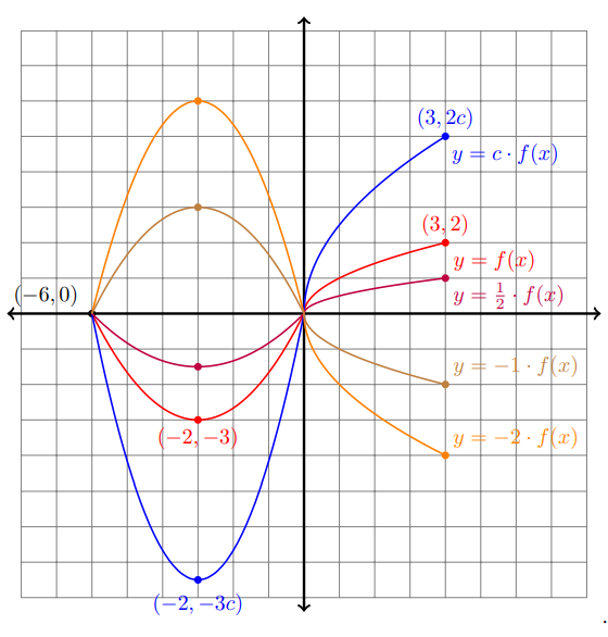
$clipboard_ee4323553c21f8ed603d1f594dd8e07ca.png$

We see from the graphs above that multiplication by a constant $y=c\cdot f(x)$ will again have the values of $x$ at each point remain the same, while the $y$-values are multiplied by $c$.

When $\textcolor{blue}{c>1}$, we get a graph which is stretched $c$ times as tall.
When $\textcolor{purple}{0<c<1}$, we get a graph which is squeezed $c$ times as tall.
When $\textcolor{brown}{c=-1}$, we reflect the graph vertically across the $x$-axis.
When $\textcolor{orange}{c<0}$, we reflect vertically and stretch/squeeze by $-c$.
All of these transformations of the graph are considered vertical stretches or reflections.

Now, we see how multiplication by a constant inside the parenthesis changes our graph $\textcolor{red}{y=f(x)}$.

$clipboard_e861157cdec7e57b708e9f98ca4f090f4.png$
We see from the graphs above that multiplication by a constant $y=f(c\cdot x)$ will again have the values of $y$ at each point remain the same, while the $x$-values are divided by $c$.
This is again because $x$ needs to compensate for the new multiplication by $c$, again making it feel 'backwards' for big and small $c$ when compared to the previous page.

When $\textcolor{blue}{0<c<1}$, we get a graph which is stretched $\frac{1}{c}$ times as wide.
When $\textcolor{purple}{c>1}$, we get a graph which is squeezed $\frac{1}{c}$ times as wide.
When $\textcolor{brown}{c=-1}$, we reflect the graph horizontally across the $y$-axis.
When $\textcolor{orange}{c<0}$, we reflect horizontally and stretch/squeeze by $-c$.
All of these transformations of the graph are considered horizontal stretches or reflections.

Individually, any of these operations (shift, stretch, or reflect) are straightforward to deal with. Sadly, in combination things can become quite complicated.

First, notice that a shift and then a stretch will give a different graph than a stretch then a shift:

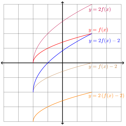
$clipboard_e9d2a241d659b38bfd2d6956c1f4de1b0.png$
Clearly, order matters when combining these transformations of graphs.
Instead of trying to keep track of many moves in order, consider this method:

If $(x_{old}, y_{old})$ are on the graph of $y=f(x)$, then $(x_{new}, y_{new})$ are on the graph of $y=\alpha f(\beta x+\gamma )+\delta $ as long as $y_{new}=\alpha y_{old}+\delta $ and $x_{old}=\beta x_{new}+\gamma $

This means we can focus on the horizontal and vertical transformations separately. If we plug in the list of known points $(x_{old},y_{old})$, we can solve these equations for the new points $(x_{new},y_{new})$. Then we can plot these points and connect the dots with the same order and shape.

Example $\PageIndex{1}$

Given the graph of $\textcolor{brown}{y=f(x)}$ below, sketch $\textcolor{purple}{y=4-3f(2-2x)}$

$clipboard_ef0941d83cc8331bb336a4379b5a06d73.png$

Solution

Our two transformation equations are $y_{new}=4-3y_{old}$ and $x_{old}=2-2x_{new}$

We plug in the $(x_{old},y_{old})$ points we know on the original graph: (-2,2), (0,0), and (2,1)

$x_{old}$	$y_{old}$	$x_{new}$	$y_{new}$
-2	2	2	-2
0	0	1	4
2	1	0	1

Now we plot these three new points $(x_{new},y_{new})$ and connect the dots in the same way to get our final graph:

$clipboard_e79761ea178a3baffd38bfa19dd01e151.png$

This page titled 1.7: Graph Transformations was last modified on Thu, 13 Mar 2025 20:04:47 GMT and is shared under a CC BY-NC-SA 4.0 license and was authored, remixed, and/or curated by Kenn Huber.

\(x_{old}\)	\(y_{old}\)	\(x_{new}\)	\(y_{new}\)
-2	2	2	-2
0	0	1	4
2	1	0	1

Contents

Text

Example \(\PageIndex{1}\)

Solution