5.10: The Ballistic Quantum Wire FET

Consider the ballistic quantum wire FET shown in Figure 5.10.1.

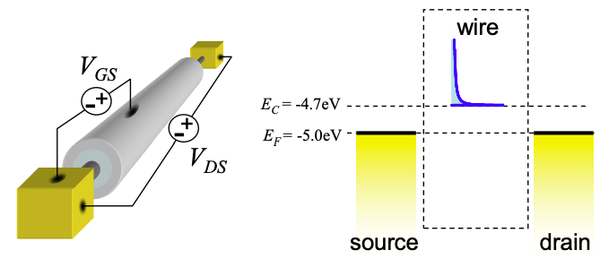
We will assume that there is only one parabolic band in the wire.

From Equation (2.10.6), the density of states in the wire is:

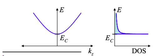
\[ g(E)dE=\frac{2L}{h}\sqrt{\frac{2m}{E-E_{C}}}u(E-E_{C})dE , \nonumber \]

where L is the length of the wire, and m is the electron mass in the wire. But only half of these states contain electrons traveling in the positive direction. Thus, we must divide Equation (5.10.1) by two to yield:

\[ g^{+}(E)dE=\frac{1}{2}\times\frac{2L}{h}\sqrt{\frac{2m}{E-E_{C}}}u(E-E_{C})dE \nonumber \]

Given the position of the Fermi Energy, this band is the conduction band. We will label the energy at the bottom of the conduction band, \(E_{C}\). Since we model electrons moving along the wire as plane waves, within the parabolic band we have

\[ E-E_{C} =\frac{\hbar^{2}k^{2}}{2m} = \frac{1}{2}mv^{2} \nonumber \]

We can rewrite Equation (5.10.2) in terms of the velocity, v, of the electron:

\[ g^{+}(E)dE = \frac{1}{2}\times \frac{4L}{hv(E)}u(E-E_{C})dE \nonumber \]

Now L/v is the transit time of an electron through the wire, thus

\[ g^{+}(E)dE = \frac{1}{2}\times \frac{4\tau(E)}{h}u(E-E_{C})dE \nonumber \]

We can substitute Equation (5.10.5) into the expression for the current density (Equation (5.9.4)) to obtain

\[ I= \frac{2q}{h}\int^{+\infty}_{-\infty} u(E-E_{C}-U)(f(E,\mu_{S})-(f(E,\mu_{D}))dE . \nonumber \]

\(^{†}\) This analysis of the ballistic quantum wire FET was introduced to me by Mark Lundstrom at Purdue University. For a complete reference see Mark Lundstrom and Jing Guo, "Nanoscale Transistors: Physics, Modeling, and Simulation‟, Springer, New York, 2006.

---