2.11: Periodic Boundary Conditions in 2-D

Applying periodic boundary conditions to 2d materials follows the same principles as in 1d.

Let's assume that the long axes of the quantum well are aligned with the x and y axes, and that the dimensions of the quantum well are \(L_{x} \times L_{y}\). When we apply periodic boundary conditions, the infinite system is periodic on both the x-axis (period \(L_{x}\)) and the y-axis (period \(L_{y}\)).

First, let's consider periodicity on the x-axis; see Figure 2.11.1.

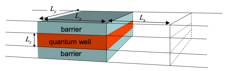
On the x-axis the wavefunction is a plane wave.

\[ \psi_{x}(x)=\text{exp}[ik_{x}x] \nonumber \]

Under periodic boundary conditions, only discrete \(k_{x}\) values are allowed

\[ k_{x}=n_{x}\frac{2\pi}{L_{x}} \nonumber \]

where \(n_{x}\) is an integer.

Similarly, for periodicity on the y-axis:

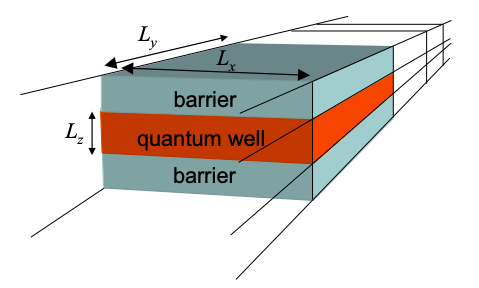
the wavefunction on the y-axis

\[ \psi_{y}y=\text{exp}[ik_{y}y] \nonumber \]

is restricted to discrete \(k_{y}\) values:

\[ k_{y}=n_{y}\frac{2\pi}{L_{y}} \nonumber \]

where \(n_{y}\) is an integer.

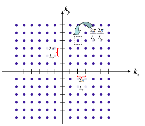
Thus, in k-space the allowed k-states are spaced regularly, with:

\[ \Delta k_{x}=\frac{2\pi}{L_{x}}, \Delta k_{y} = \frac{2\pi}{L_{y}} \nonumber \]

Overall, the area occupied in k-space per k-state is:

\[ \Delta k^{2} = \Delta k_{x}\Delta k_{y} =\frac{2\pi}{L_{x}}\frac{2\pi}{L_{y}}= \frac{4\pi^{2}}{A} \nonumber \]

where A is the area of the quantum well.

---