Opening the book…
- Chapter 1: The Chemical World
- 1.1: The Scope of Chemistry
- 1.2: Chemicals Compose Ordinary Things
- 1.3: Hypothesis, Theories, and Laws
- 1.4: The Scientific Method: How Chemists Think
- 1.5: A Beginning Chemist: How to Succeed
- Chapter 2: Measurement and Problem Solving
- 2.1: Taking Measurements
- 2.2: Scientific Notation: Writing Large and Small Numbers
- 2.3: Significant Figures: Writing Numbers to Reflect Precision
- 2.4: Significant Figures in Calculations
- 2.5: The Basic Units of Measurement
- 2.6: Problem Solving and Unit Conversions
- 2.7: Solving Multistep Conversion Problems
- 2.8: Units Raised to a Power
- 2.9: Density
- 2.10: Numerical Problem-Solving Strategies and the Solution Map
- 2.E: Measurement and Problem Solving (Exercises)
- Chapter 3: Matter and Energy
- 3.1: In Your Room
- 3.2: What is Matter?
- 3.3: Classifying Matter According to Its State: Solid, Liquid, and Gas
- 3.4: Classifying Matter According to Its Composition
- 3.5: Differences in Matter: Physical and Chemical Properties
- 3.6: Changes in Matter: Physical and Chemical Changes
- 3.7: Conservation of Mass: There is No New Matter
- 3.8: Energy
- 3.9: Energy and Chemical and Physical Change
- 3.10: Temperature: Random Motion of Molecules and Atoms
- 3.11: Temperature Changes: Heat Capacity
- 3.12: Energy and Heat Capacity Calculations
- 3.E: Exercises
- Chapter 4: Atoms and Elements
- 4.1: Experiencing Atoms at Tiburon
- 4.2: Indivisible: The Atomic Theory
- 4.3: The Nuclear Atom
- 4.4: The Properties of Protons, Neutrons, and Electrons
- 4.5: Elements: Defined by Their Numbers of Protons
- 4.6: Looking for Patterns: The Periodic Law and the Periodic Table
- 4.7: Ions: Losing and Gaining Electrons
- 4.8: Isotopes: When the Number of Neutrons Varies
- 4.9: Atomic Mass: The Average Mass of an Element’s Atoms
- Chapter 5: Molecules and Compounds
- 5.1: Sugar and Salt
- 5.2: Compounds Display Constant Composition
- 5.3: Chemical Formulas: How to Represent Compounds
- 5.4: A Molecular View of Elements and Compounds
- 5.5: Writing Formulas for Ionic Compounds
- 5.6: Nomenclature: Naming Compounds
- 5.7: Naming Ionic Compounds
- 5.8: Naming Molecular Compounds
- 5.9: Naming Acids
- 5.10: Nomenclature Summary
- 5.11: Formula Mass: The Mass of a Molecule or Formula Unit
- Chapter 6: Chemical Composition
- 6.1: How Much Sodium?
- 6.2: Counting Nails by the Pound
- 6.3: Counting Atoms by the Gram
- 6.4: Counting Molecules by the Gram
- 6.5: Chemical Formulas as Conversion Factors
- 6.6: Mass Percent Composition of Compounds
- 6.7: Mass Percent Composition from a Chemical Formula
- 6.8: Calculating Empirical Formulas for Compounds
- 6.9: Calculating Molecular Formulas for Compounds
- Chapter 7: Chemical Reactions
- 7.1: Grade School Volcanoes, Automobiles, and Laundry Detergents
- 7.2: Evidence of a Chemical Reaction
- 7.3: The Chemical Equation
- 7.4: How to Write Balanced Chemical Equations
- 7.5: Aqueous Solutions and Solubility: Compounds Dissolved in Water
- 7.6: Precipitation Reactions: Reactions in Aqueous Solution That Form a Solid
- 7.7: Writing Chemical Equations for Reactions in Solution: Molecular, Complete Ionic, and Net Ionic Equations
- 7.8: Acid–Base and Gas Evolution Reactions
- 7.9: Oxidation–Reduction Reactions
- 7.10: Classifying Chemical Reactions
- 7.11: The Activity Series
- Chapter 8: Quantities in Chemical Reactions
- 8.1: Climate Change: Too Much Carbon Dioxide
- 8.2: Stoichiometry
- 8.3: Making Molecules: Mole-to-Mole Conversions
- 8.4: Making Molecules: Mass-to-Mass Conversions
- 8.5: Limiting Reactant, Theoretical Yield, and Percent Yield
- 8.6: Limiting Reactant, Theoretical Yield, and Percent Yield from Initial Masses of Reactants
- 8.7: Enthalpy: A Measure of the Heat Evolved or Absorbed in a Reaction
- Chapter 9: Electrons in Atoms and the Periodic Table
- 9.1: Blimps, Balloons, and Models of the Atom
- 9.2: Light: Electromagnetic Radiation
- 9.3: The Electromagnetic Spectrum
- 9.4: The Bohr Model: Atoms with Orbits
- 9.5: The Quantum-Mechanical Model: Atoms with Orbitals
- 9.6: Quantum-Mechanical Orbitals and Electron Configurations
- 9.7: Electron Configurations and the Periodic Table
- 9.8: The Explanatory Power of the Quantum-Mechanical Model
- 9.9: Periodic Trends: Atomic Size, Ionization Energy, and Metallic Character
- Chapter 10: Chemical Bonding
- 10.1: Bonding Models and AIDS Drugs
- 10.2: Representing Valence Electrons with Dots
- 10.3: Lewis Structures of Ionic Compounds: Electrons Transferred
- 10.4: Covalent Lewis Structures: Electrons Shared
- 10.5: Writing Lewis Structures for Covalent Compounds
- 10.6: Resonance: Equivalent Lewis Structures for the Same Molecule
- 10.7: Predicting the Shapes of Molecules
- 10.8: Electronegativity and Polarity: Why Oil and Water Don’t Mix
- Chapter 11: Gases
- 11.1: Extra-Long Straws
- 11.2: Kinetic Molecular Theory: A Model for Gases
- 11.3: Pressure: The Result of Constant Molecular Collisions
- 11.4: Boyle’s Law: Pressure and Volume
- 11.5: Charles’s Law: Volume and Temperature
- 11.6: Gay-Lussac's Law: Temperature and Pressure
- 11.7: The Combined Gas Law: Pressure, Volume, and Temperature
- 11.8: Avogadro’s Law: Volume and Moles
- 11.9: The Ideal Gas Law: Pressure, Volume, Temperature, and Moles
- 11.10: Mixtures of Gases: Why Deep-Sea Divers Breathe a Mixture of Helium and Oxygen
- 11.11: Gases in Chemical Reactions
- Chapter 12: Liquids, Solids, and Intermolecular Forces
- 12.1: Interactions between Molecules
- 12.2: Properties of Liquids and Solids
- 12.3: Intermolecular Forces in Action: Surface Tension and Viscosity
- 12.4: Evaporation and Condensation
- 12.5: Melting, Freezing, and Sublimation
- 12.6: Types of Intermolecular Forces: Dispersion, Dipole–Dipole, Hydrogen Bonding, and Ion-Dipole
- 12.7: Types of Crystalline Solids: Molecular, Ionic, and Atomic
- 12.8: Water: A Remarkable Molecule
- Chapter 13: Solutions
- 13.1: Prelude - Tragedy in Cameroon
- 13.2: Solutions: Homogeneous Mixtures
- 13.3: Solutions of Solids Dissolved in Water: How to Make Rock Candy
- 13.4: Solutions of Gases in Water: How Soda Pop Gets Its Fizz
- 13.5: Solution Concentration: Mass Percent
- 13.6: Solution Concentration: Molarity
- 13.7: Solution Dilution
- 13.8: Solution Stoichiometry
- 13.9: Freezing Point Depression and Boiling Point Elevation: Making Water Freeze Colder and Boil Hotter
- 13.10: Osmosis: Why Drinking Salt Water Causes Dehydration
- Chapter 14: Acids and Bases
- 14.1: Sour Patch Kids and International Spy Movies
- 14.2: Acids: Properties and Examples
- 14.3: Bases: Properties and Examples
- 14.4: Molecular Definitions of Acids and Bases
- 14.5: Reactions of Acids and Bases
- 14.6: Acid–Base Titration: A Way to Quantify the Amount of Acid or Base in a Solution
- 14.7: Strong and Weak Acids and Bases
- 14.8: Water: Acid and Base in One
- 14.9: The pH and pOH Scales: Ways to Express Acidity and Basicity
- 14.10: Buffers: Solutions That Resist pH Change
- To convert a value reported in one unit to a corresponding value in a different unit using conversion factors.
During your studies of chemistry (and physics also), you will note that mathematical equations are used in many different applications. Many of these equations have a number of different variables with which you will need to work. You should also note that these equations will often require you to use measurements with their units. Algebra skills become very important here!
Converting Between Units with Conversion Factors
A conversion factor is a factor used to convert one unit of measurement into another. A simple conversion factor can convert meters into centimeters, or a more complex one can convert miles per hour into meters per second. Since most calculations require measurements to be in certain units, you will find many uses for conversion factors. Always remember that a conversion factor has to represent a fact; this fact can either be simple or more complex. For instance, you already know that 12 eggs equal 1 dozen. A more complex fact is that the speed of light is \(1.86 \times 10^5\) miles/\(\text{sec}\). Either one of these can be used as a conversion factor depending on what type of calculation you are working with (Table \(\PageIndex{1}\)).
| English Units | Metric Units | Quantity |
|---|---|---|
| 1 ounce (oz) | 28.35 grams (g) | *mass |
| 1 fluid once (oz) | 29.6 mL | volume |
| 2.205 pounds (lb) | 1 kilogram (kg) | *mass |
| 1 inch (in) | 2.54 centimeters (cm) | length |
| 0.6214 miles (mi) | 1 kilometer (km) | length |
| 1 quarter (qt) | 0.95 liters (L) | volume |
*Pounds and ounces are technically units of force, not mass, but this fact is often ignored by the non-scientific community.
Of course, there are other ratios which are not listed in Table \(\PageIndex{1}\). They may include:
- Ratios embedded in the text of the problem (using words such as per or in each, or using symbols such as / or %).
- Conversions in the metric system, as covered earlier in this chapter.
- Common knowledge ratios (such as 60 seconds \(=\) 1 minute).
If you learned the SI units and prefixes described, then you know that 1 cm is 1/100th of a meter.
\[ 1\; \rm{cm} = \dfrac{1}{100} \; \rm{m} = 10^{-2}\rm{m} \nonumber \]
or
\[100\; \rm{cm} = 1\; \rm{m} \nonumber \]
Suppose we divide both sides of the equation by \(1 \text{m}\) (both the number and the unit):
\[\mathrm{\dfrac{100\:cm}{1\:m}=\dfrac{1\:m}{1\:m}} \nonumber \]
As long as we perform the same operation on both sides of the equals sign, the expression remains an equality. Look at the right side of the equation; it now has the same quantity in the numerator (the top) as it has in the denominator (the bottom). Any fraction that has the same quantity in the numerator and the denominator has a value of 1:
\[ \dfrac{ \text{100 cm}}{\text{1 m}} = \dfrac{ \text{1000 mm}}{\text{1 m}}= \dfrac{ 1\times 10^6 \mu \text{m}}{\text{1 m}}= 1 \nonumber \]
We know that 100 cm is 1 m, so we have the same quantity on the top and the bottom of our fraction, although it is expressed in different units.
Performing Dimensional Analysis
Dimensional analysis is amongst the most valuable tools that physical scientists use. Simply put, it is the conversion between an amount in one unit to the corresponding amount in a desired unit using various conversion factors. This is valuable because certain measurements are more accurate or easier to find than others. The use of units in a calculation to ensure that we obtain the final proper units is called dimensional analysis.
Here is a simple example. How many centimeters are there in 3.55 m? Perhaps you can determine the answer in your head. If there are 100 cm in every meter, then 3.55 m equals 355 cm. To solve the problem more formally with a conversion factor, we first write the quantity we are given, 3.55 m. Then we multiply this quantity by a conversion factor, which is the same as multiplying it by 1. We can write 1 as \(\mathrm{\dfrac{100\:cm}{1\:m}}\) and multiply:
\[ 3.55 \; \rm{m} \times \dfrac{100 \; \rm{cm}}{1\; \rm{m}} \nonumber \]
The 3.55 m can be thought of as a fraction with a 1 in the denominator. Because m, the abbreviation for meters, occurs in both the numerator and the denominator of our expression, they cancel out:
\[\dfrac{3.55 \; \cancel{\rm{m}}}{ 1} \times \dfrac{100 \; \rm{cm}}{1 \; \cancel{\rm{m}}} \nonumber \]
The final step is to perform the calculation that remains once the units have been canceled:
\[ \dfrac{3.55}{1} \times \dfrac{100 \; \rm{cm}}{1} = 355 \; \rm{cm} \nonumber \]
In the final answer, we omit the 1 in the denominator. Thus, by a more formal procedure, we find that 3.55 m equals 355 cm. A generalized description of this process is as follows:
quantity (in old units) × conversion factor = quantity (in new units)
You may be wondering why we use a seemingly complicated procedure for a straightforward conversion. In later studies, the conversion problems you encounter will not always be so simple. If you master the technique of applying conversion factors, you will be able to solve a large variety of problems.
In the previous example, we used the fraction \(\dfrac{100 \; \rm{cm}}{1 \; \rm{m}}\) as a conversion factor. Does the conversion factor \(\dfrac{1 \; \rm m}{100 \; \rm{cm}}\) also equal 1? Yes, it does; it has the same quantity in the numerator as in the denominator (except that they are expressed in different units). Why did we not use that conversion factor? If we had used the second conversion factor, the original unit would not have canceled, and the result would have been meaningless. Here is what we would have gotten:
\[ 3.55 \; \rm{m} \times \dfrac{1\; \rm{m}}{100 \; \rm{cm}} = 0.0355 \dfrac{\rm{m}^2}{\rm{cm}} \nonumber \]
For the answer to be meaningful, we have to construct the conversion factor in a form that causes the original unit to cancel out. Figure \(\PageIndex{1}\) shows a concept map for constructing a proper conversion.
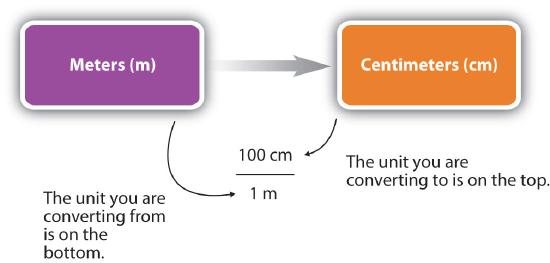
- Identify the "given" information in the problem. Look for a number with units to start this problem with.
- What is the problem asking you to "find"? In other words, what unit will your answer have?
- Use ratios and conversion factors to cancel out the units that aren't part of your answer, and leave you with units that are part of your answer.
- When your units cancel out correctly, you are ready to do the math. You are multiplying fractions, so you multiply the top numbers and divide by the bottom numbers in the fractions.
Significant Figures in Conversions
How do conversion factors affect the determination of significant figures?
- Numbers in conversion factors based on prefix changes, such as kilograms to grams, are not considered in the determination of significant figures in a calculation because the numbers in such conversion factors are exact.
- Exact numbers are defined or counted numbers, not measured numbers, and can be considered as having an infinite number of significant figures. (In other words, 1 kg is exactly 1,000 g, by the definition of kilo-.)
- Counted numbers are also exact. If there are 16 students in a classroom, the number 16 is exact.
- In contrast, conversion factors that come from measurements (such as density, as we will see shortly) or that are approximations have a limited number of significant figures and should be considered in determining the significant figures of the final answer.
| Example \(\PageIndex{1}\) | Example \(\PageIndex{2}\) | |
|---|---|---|
| Steps for Problem Solving | The average volume of blood in an adult male is 4.7 L. What is this volume in milliliters? | A hummingbird can flap its wings once in 18 ms. How many seconds are in 18 ms? |
| Identify the "given" information and what the problem is asking you to "find." | Given: 4.7 L Find: mL |
Given: 18 ms Find: s |
| List other known quantities. | \(1\, mL = 10^{-3} L \) | \(1 \,ms = 10^{-3} s \) |
| Prepare a concept map and use the proper conversion factor. |  |
 |
| Cancel units and calculate. |
\( 4.7 \cancel{\rm{L}} \times \dfrac{1 \; \rm{mL}}{10^{-3}\; \cancel{\rm{L}}} = 4,700\; \rm{mL}\) \( 4.7 \cancel{\rm{L}} \times \dfrac{1,000 \; \rm{mL}}{1\; \cancel{\rm{L}}} = 4,700\; \rm{mL}\) or 4.7 x 10³ 2SF, not ambiguous |
\( 18 \; \cancel{\rm{ms}} \times \dfrac{10^{-3}\; \rm{s}}{1 \; \cancel{\rm{ms}}} = 0.018\; \rm{s}\) or \( 18 \; \cancel{\rm{ms}} \times \dfrac{1\; \rm{s}}{1,000 \; \cancel{\rm{ms}}} = 0.018\; \rm{s}\) |
| Think about your result. | The amount in mL should be 1000 times larger than the given amount in L. | The amount in s should be 1/1000 the given amount in ms. |
Perform each conversion.
- 101,000 ns to seconds
- 32.08 kg to grams
- 1.53 grams to cg
- Answer a:
- \(1.01000 x 10^{-4} s \)
- Answer b:
- \(3.208 x 10^{4} g \)
- Answer c:
- \(1.53 x 10^{2} cg \)
Summary
- Conversion factors are used to convert one unit of measurement into another.
- Dimensional analysis (unit conversions) involves the use of conversion factors that will cancel unwanted units and produce the appropriate units.
2.6: Problem Solving and Unit Conversions is shared under a CC BY-NC-SA 4.0 license and was authored, remixed, and/or curated by LibreTexts.
The book could not be loaded just now.