Opening the book…
Introduction
The canonical expressions for thermodynamic quantities require calculating Q. We want to be able to use what we know about the microscopic (quantum) behavior of molecules to do this. Thus, we need to connect Q to the microscopic (quantum) energy levels. The microcanonical q is defined it in terms of the energy levels of the molecules in the system. So, our goal is to determine the connection between the two partition functions.
Total energy of a system
To make our notation more compact we will use the common formalism of using the substitution \(\beta = \frac{1}{k_B T}\).
A system, such as a container of gas, can consist of a large number of particles. Their energies are additive so in a sytem with total energy Ei:
\[E_i = \epsilon_i(1) + \epsilon_i(2) + \epsilon_i(3) + \cdots \nonumber \]
Each of the molecules can have their energy distributed over their respective internal energy states (e.g., vibrations, rotations, etc.). This means that each \(\epsilon_i(k)\) is already a summation over the states of the molecule. Thus,
\[E_i = \sum_{i,k,j}\epsilon_{i,k,j},\nonumber\]
where i is the canonical energy index, k indicates the particle and j the energy state of the particle.
Q versus q
When calculating Q it should not matter which order we sum over the possible energy combinations of quantum levels, just that we include them all. Thus, assuming all the molecules are distinguishable (e.g. in a crystal they could be identified by position), we can get the canonical partition function as:
\[Q(N,V,\beta) = \sum_i e^{-\beta E_i} = \sum_{i} exp\left({-\beta \sum_{j,k}\epsilon_{i,j,k}}\right). \nonumber \]
Because it does not matter whether we sum over the states of the system or all the individual states of the molecules we can instead write this as the product of the sums for each of the molecules:
\[Q(N, V, \beta) = \left(\sum_j e^{\beta \epsilon_j}\right)\left(\sum_j e^{\beta \epsilon_j}\right)\left(\sum_j e^{\beta \epsilon_j}\right)...\nonumber\]
Where each factor is for a different molecule (different k). Each of the sums is a microcanonical q, where the summation is over molecular energy states rather than system energies of a canonical ensemble. So, compactly we have:
\[Q(N,V,\beta) = \prod_k{q_k} \nonumber \]
If the energy states of all the particles are the same, then the equation simplifies to:
\[ Q(N,V,\beta) = [q(V,\beta)]^N \label{Qdist} \]
We can do this if, for example, the particles are embedded in a crystal where we can distinguish them by their location.
However, under most conditions, full knowledge of each member of an ensemble is missing and hence we have to operate with a more reduced knowledge. This is demonstrated via a simple model of two particles in a two-energy level system in Figure \(\PageIndex{1}\). Each particle (red or blue) can occupy either the \(E_1=0\) energy level or the \(E_2=\epsilon\) energy level resulting in four possible states that describe the system. The corresponding partition function for this system is then:
\[Q_{\text{distinguishable}}=e^0+ e^{-\beta\epsilon} + e^{-\beta\epsilon} + e^{-2 \beta\epsilon}=q^2 \label{Q1} \]
and is just the molecular partition function (\(q\)) squared.
\[q^2 = q_{blue}q_{red} = (e^0 + e^{-\beta\epsilon}) (e^0 + e^{-\beta\epsilon})\nonumber\]
because each particle can occupy either the 0 or \(\epsilon\) state.
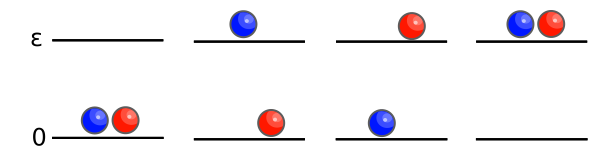
However, if the two particles are indistinguishable (e.g., both the same color as in Figure \(\PageIndex{2}\)) then while four different combinations can be generated like in Figure \(\PageIndex{1}\), there is no discernible way to separate the two middle states. Hence, there are effectively only three states observable for this system.

The corresponding partition function for this system can be constructed:
\[ Q(N,V,\beta) =e^0+ e^{-\beta\epsilon} + e^{-2 \beta\epsilon} \neq q^2 \label{Q2} \]
and this is not equal to the square of the molecular partition function. If Equation \ref{Qdist} were used to describe the indistinguishable particle case, then it would overestimate the number of observable states. From combinatorics, using \(q^N\) for a large \(N\)-particle system of indistinguishable particles will overestimate the number of states by a factor of \(N!\). Therefore Equation \ref{Q1} requires a slight modification to account for this over counting.
\[ Q(N,V,\beta) = \dfrac{\sum_i{e^{-\beta E_i}}}{N!} \label{2} \]
If we have \(N\) molecules, we can perform \(N!\) permutations that should not affect the outcome. To avoid over counting (making sure we do not count each state more than once), the partition function becomes:
\[Q(N,V,\beta) = \dfrac{q(V,\beta)^N}{N!} \label{Qindist} \]
As you may have noticed, using Equation \ref{2} to estimate of \(Q\) for the two-indistinguishable particle discussed case above with \(N=2\) is incorrect (i.e., Equation \ref{2} is not equal to Equation \ref{Q2}). That is because the \(N!\) factor is only applicable for large \(N\).
This page titled 2.3: Microconanonical (q molecular) Versus Canonical (Q) Partition Functions was last modified on Wed, 17 Sep 2025 19:10:19 GMT and is shared under a CC BY-NC-SA 4.0 license and was authored, remixed, and/or curated by Jonathan Gutow.
The book could not be loaded just now.