10.1.1: The Idea of Dynamic Chemical Equilibrium

Reversible Reactions and Equilibrium

Consider the hypothetical reaction:

\[\text{A} + \text{B} \rightarrow \text{C} + \text{D}. \nonumber \]

If we looked at this reaction using what we have learned, this reaction will keep going, forming \(\text{C}\) and \(\text{D}\) until \(\text{A}\) and \(\text{B}\) run out. This is what we call an "irreversible reaction" or a "reaction that goes to completion".

Some reactions, however, are reversible, meaning the reaction can go backwards in which products react to form reactants, so that: \(\text{A} + \text{B} \leftarrow \text{C} + \text{D}\). The direction of the arrow shows that \(\text{C}\) and \(\text{D}\) are reacting to form \(\text{A}\) and \(\text{B}\). What if the two reactions, the forward reaction and the reverse reaction, were occurring at the same time? What would this look like? If you could peer into the reaction, you would be able to find \(\text{A}\), \(\text{B}\), \(\text{C}\), and \(\text{D}\) particles. \(\text{A}\) and \(\text{B}\) would react to form \(\text{C}\) and \(\text{D}\) at the same time that \(\text{C}\) and \(\text{D}\) are reacting to form \(\text{A}\) and \(\text{B}\).

If the forward and reverse reactions are happening at the same rate, the reaction is said to be at equilibrium or dynamic equilibrium. At this point, the concentrations of \(\text{A}\), \(\text{B}\), \(\text{C}\), and \(\text{D}\) are not changing (or, are constant) and we would see no difference in our reaction container, but reactions are still occurring in both directions. It is important to point out that having constant amounts of reactants and products does NOT mean that the concentration of the reactants is equal to the concentration of the products. It means they are not changing. These reactions appear to have stopped before one of the reactants has run out.

Chemists use a double-headed arrow, \(\rightleftharpoons\), to show that a reaction is at equilibrium. We would write the example reaction as:

\[\text{A} + \text{B} \rightleftharpoons \text{C} + \text{D}. \nonumber \]

The arrow indicates that both directions of the reaction are happening.

Another way to think about reversible and irreversible reactions is to compare them to two types of games of tag. Reversible reactions are in many ways like a traditional game of tag: the "it" person can become "not it" and somebody who is "not it" is tagged and becomes "it". In this way, it is a reversible change. It is also like a reaction at equilibrium, because overall no change is occurring. There is always a constant number of "it" people and "not it" people in the game. Also, having constant numbers of "it" and "not it" people in our game does not mean that the number of "it" people (reactants) is equal to the number of "not it" people (products). Furthermore, this is similar to equilibrium in that this game never truly ends (unless everybody gets tired of playing). The game could go on forever. We could write this as the following reversible reaction:

\[\text{"It"} \rightleftharpoons \text{"Not it"} \nonumber \]

Irreversible reactions (those that only go in one direction from reactants to products and cannot reach a state of equilibrium) are more like a game of sharks and minnows. In sharks and minnows, almost everybody starts out as a minnow. Once tagged, they become a shark. However, the difference here is that once you are a shark you are always a shark; there is no way to go back to becoming a minnow. The game continues until everybody has been tagged and becomes a shark. This is similar to irreversible reactions in that the reactants turn into products, but can't change back. Furthermore, the reaction will proceed until the reactants have been used up and there are not any more left. We could write the reaction as:

\[\text{Minnow} \rightarrow \text{Shark} \nonumber \]

Here's another example of a reversible reaction—dissolving salt in a beaker of water, described by the following reaction:

\[\ce{NaCl(s) \leftrightarrow NaCl(aq)} \nonumber \]

If you keep adding more and more solid salt, eventually you'll reach the point where no more salt dissolves, and the excess sits at the bottom of the beaker. At this point we have a saturated solution. Has the dissolving reaction stopped? It would appear so, but that's not the case (wouldn't that be too easy?).

What happens in our saturated solution, which has reached the point of equilibrium, is that both the forward

\[\ce{NaCl(s) \rightarrow NaCl(aq)} \nonumber \]

and reverse

\[\ce{NaCl(aq) \rightarrow NaCl(s)} \nonumber \]

reactions are still going on, but at the same rate. This in effect cancels out any observable, or measurable, changes in our system. At the same rate that solid NaCl produces aqueous NaCl (dissolved salt), the dissolved salt is re-crystallizing to form more solid NaCl.

• Equilibrium is the state at which the rate of the forward reaction equals the rate of the reverse reaction.
• At the point of equilibrium, no more measurable or observable changes in the system can be noted.

It is important for you to understand that equilibrium means the rates of the forward and reverse reactions are equal; it does not mean that there are equal amounts of reactants and products present at equilibrium.

For example, the following reaction was allowed to come to the point of equilibrium, and concentrations of all reaction participants were measured at that time:

\(\ce{H_2(g) + I_2(g) \leftrightarrow 2HI(g)}\)

At equilibrium:	\(\mathrm{[H_2]=0.022\: M}\) \(\mathrm{[I_2]=0.022\: M}\) \(\mathrm{[HI]=0.156\: M}\)

For this particular reversible reaction, there is more HI at equilibrium (0.156 M) than there is of H₂ and I₂ (both at 0.022M). We say that the product side of the reaction is favored.

Equilibrium does not mean equal amounts at equilibrium!

Here is an example to help you understand how equilibrium works: imagine yourself on a escalator that is going down. You start at the top (reactants) and end up at the bottom (products). But when you are partway down, you start walking up the escalator as it continues going down. If you match your rate of walking up to the same rate that the escalator is going down, you make no progress and appear to be at a standstill. To an observer it would look as if you and the escalator had come to a stop, when actually both upward and downward movements continue.

Equilibrium is dynamic—both forward and reverse reactions continue, even though the reaction appears to have stopped. And this equilibrium does not need to occur right in the middle of two floors—you could be near the bottom, near the top, or anywhere in between when you carry out your reverse process.

In order for a reversible reaction to reach the point of equilibrium, the reaction must be carried out in a closed system—no additional reactants can be added or products removed. If, in our last example, the product HI was removed as it formed, the reaction would never reach the point of equilibrium; instead, H₂ and I₂ would continue to react to produce HI until one or both of the reactants was used up.

If reactants are constantly being added, and products removed as they form, the system would appear to be at equilibrium because to an outside observer it would appear that the reaction has stopped—but that would not be the case. This situation—with new material constantly being added as products are removed—is called a steady state system. A factory with an assembly line is a steady state system—new raw materials are constantly being added; finished products are removed. A campfire with wood being added to the fire is another steady state system. Be careful not to confuse steady state with equilibrium.

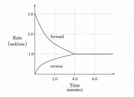
How do the rates of the forward and reverse reactions change as the reaction heads towards equilibrium (before it reaches equilibrium)?

If we start our above reaction with H₂ and I₂, and with no HI, the two gases will react at a certain rate. But remember that the rate of a reaction slows down over time, as the reactants get used up (and lower their concentrations). Eventually, however, the amount of the product HI increases, and it will begin producing H₂ and I₂. Thus the rate of the reverse reaction starts out slowly (there is no HI present), but will speed up as the concentration of HI increases. Eventually both rates will level off (not always to the same level as shown by this example, however):

Chemists have found that there is a mathematical relationship that exists between the concentration of the reactants and products, once equilibrium has been reached, that is independent of the initial concentration of the participants. For any general reaction,

\[\ce{aA + bB \rightleftharpoons cD + dD} \label{2.1.1} \]

an equilibrium constant expression can be written as:

\[\mathrm{K_{eq}=\dfrac{[C]^c \times [D]^d}{[A]^a \times [B]^b}} \label{2.1.2} \]

This mathematical relationship exists for all equilibrium systems, and produces a constant ratio called the equilibrium constant, K_eq .

Law of Mass-Action

Equation \ref{2.1.2} is sometimes called the Law of Mass-Action.

This relationship will be very important to us for the next few units, so it is important that you understand how to set this relationship up and what it tells us about an equilibrium system.

The products of the reaction (C and D) are placed in the numerator, and their concentrations are raised to the power of the coefficients from the balanced equation. The reactants (A and B) are placed in the denominator, with their concentrations raised to the power of their coefficients.

Example \(\PageIndex{1}\)

For the reaction between hydrogen and iodine gas to produce hydrogen iodide:

\[\ce{H_2(g) + I_2(g) \rightleftharpoons 2HI(g)} \label{2.1.3} \]

the equilibrium constant expression will be:

\[\mathrm{K_{eq}=\dfrac{[HI]^2}{[H_2] \times [I_2]}} \label{2.1.4} \]

Using the example we examined in our last section, equilibrium concentrations for each substance were measured at equilibrium and found to be:

At equilibrium:	\(\mathrm{[H_2]=0.022\: M}\) \(\mathrm{[I_2]=0.022\: M}\) \(\mathrm{[HI]=0.156\: M}\)

We substitute these values into our equilibrium expression and solve for K_eq:

\[\mathrm{K_{eq}=\dfrac{[HI]^2}{[H_2] \times [I_2]}=\dfrac{(0.156)^2}{(0.022)(0.022)}=50.3} \nonumber \]

The value of K_eq, which has no units, is a constant for any particular reaction, and its value does not change unless the temperature of the system is changed. It does not depend on the initial concentrations used to reach the point of equilibrium.

For example, the following data were obtained for equilibrium concentrations of H₂, I₂ and HI, and the value of K_eq was calculated for each trial:

Trial

Aside from accounting for slight experimental variation between trials, the value for K_eq is the same despite differences in equilibrium concentrations for the individual participants.

There is one other important point to make at this time.

K_eq relates the concentrations of products to reactants at equilibrium.

For aqueous solutions, concentration is often measured as mol · L^-1. For gases, concentration is often measured as partial pressure.

The concentrations of both aqueous solutions and gases change during the progress of a reaction. For reactions involving a solid or a liquid, while the amounts of the solid or liquid will change during a reaction, their concentrations (much like their densities) will not change during the reaction. Instead, their values will remain constant. Because they are constant, their values are not included in the equilibrium constant expression.

Example \(\PageIndex{2}\)

For example, consider the reaction showing the formation of solid calcium carbonate from solid calcium oxide and carbon dioxide gas:

\[\ce{CaO(s) + CO_2(g) \leftrightarrow CaCO_3(s)} \nonumber \]

The equilibrium constant for this reaction is (before modification):

\[\mathrm{K_{eq}=\dfrac{[CaCO_3]}{[CaO] \times [CO_2]}} \nonumber \]

But we remove those participants whose state is either a solid or a liquid, which leaves us with the following equilibrium constant expression:

\[\mathrm{K_{eq}=\dfrac{1}{[CO_2]}} \nonumber \]

Summary

• There are a few possible ways a reaction can go: it can go to completion (\(\text{reactants} \rightarrow \text{products}\)), and it can occur but not go to completion. Instead, it will reach chemical equilibrium (\(\text{reactants} \rightleftharpoons \text{products}\)).
• Chemical equilibrium occurs when the number of particles becoming products is equal to the number of particles becoming reactants.
• A dynamic equilibrium is a state where the rate of the forward reaction is equal to the rate of the reverse reaction.

Vocabulary

• Equilibrium - A state that occurs when the rate of the forward reaction is equal to the rate of the reverse reaction.