Opening the book…
- Explain steady state and steady-state approximation.
- Derive a rate law when a mechanism is given but the rate determining step is not identified.
- Derive a general expression of the rate law using the steady-state approximation.
- Make appropriate assumptions so that the derived rate law agrees with the observed rate law.
- Give expressions for the producing rate of an intermediate.
- Give expressions for the consuming rate of an intermediate.
- Express concentration of intermediate in terms of concentration of reactants.
- Eliminate concentrations of intermediates using concentrations of reactants.
- Derive a rate law from the many elementary steps.
- Discuss the derived rate law.
The Steady-State Approximation
When a reaction mechanism has several steps of comparable rates, the rate-determining step is often not obvious. However, there is an intermediate in some of the steps. An intermediate is a species that is neither one of the reactants, nor one of the products. The steady-state approximation is a method used to derive a rate law. The method is based on the assumption that one intermediate in the reaction mechanism is consumed as quickly as it is generated. Its concentration remains the same in a duration of the reaction.
An intermediate is a species that is neither one of the reactants, nor one of the products. It transiently exists during the course of the reaction.
When a reaction involves one or more intermediates, the concentration of one of the intermediates remains constant at some stage of the reaction. Thus, the system has reached a steady-state. The concentration of one of the intermediates, \([Int]\), varies with time as shown in Figure \(\PageIndex{1}\). At the start and end of the reaction, [Int] does vary with time.
\[ \dfrac{d[Int]}{dt}= 0 \nonumber \]
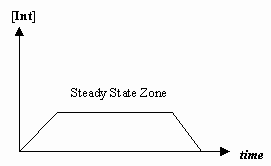
When a reaction mechanism has several steps with comparable rates, the rate-determining step is not obvious. However, there is an intermediate in some of the steps. The steady-state approximation implies that you select an intermediate in the reaction mechanism, and calculate its concentration by assuming that it is consumed as quickly as it is generated. In the following, an example is given to show how the steady-state approximation method works.
The Lindemann mechanism, sometimes called the Lindemann-Hinshelwood mechanism, is a schematic reaction mechanism. Frederick Lindemann discovered the concept in 1921 and Cyril Hinshelwood developed it. It breaks down a stepwise reaction into two or more elementary steps, then it gives a rate constant for each elementary step. The rate law and rate equation for the entire reaction can be derived from this information. Lindemann mechanisms have been used to model gas phase decomposition reactions. Although the net formula for a decomposition may appear to be first-order (unimolecular) in the reactant, a Lindemann mechanism may show that the reaction is actually second-order (bimolecular).
A Lindemann mechanism typically includes an activated reaction intermediate, labeled A* (where A can be any element or compound). The activated intermediate is produced from the reactants only after a sufficient activation energy is applied. It then either deactivates from A* back to A, or reacts with another (dis)similar reagent to produce yet another reaction intermediate or the final product P.
Use the steady-state approximation to derive the rate law for this reaction
\[\ce{A \rightarrow P}\nonumber \]
assuming it follows the following two-step mechanism:
\[\begin{align} \ce{ A + M } &\underset{\Large{k_{\textrm -1}}}{\overset{\Large{k_{\textrm 1}}}\rightleftharpoons} \ce{A^{\ast} + M} \tag{step 1} \\[4pt] \ce{A^{\ast}} &\ce{->[\large{k_2}] P } \tag{step 2} \end{align} \]
M = a bath gas or third body — any molecule (e.g., N2, Ar, or even the same species A) that collides with A to transfer energy, while remaining chemically unchanged.
Assuming that the concentration of intermediate A* is held constant according to the quasi steady-state approximation, what is the rate of formation of product P?
Solution
First, find the rates of production and consumption of intermediate A*. The rate of production of A* in the first elementary step (step 1) and A* is consumed both in the reverse first step and in the forward second step.
\(\ce{production\: rate\: of\: A^{\ast}} = k_1 \ce{[A] [M]}\)
\(\ce{consumption\: rate\: of\: A^{\ast}} = k_{-1} \ce{[A^{\ast}] [M]} + k_2 \ce{[A^{\ast}] } \)
A steady-state approach makes use of the assumption that the rate of production of an intermediate is equal to the rate of its consumption. Thus, we have
\(k_1 \ce{[A] [M]} = k_{-1} \ce{[A^{\ast}] [M]} + k_2 \ce{[A^{\ast}] } \)
and solving for \(\ce{[A^{\ast}]}\) gives the result,
\[ \ce{[A^{\ast}]} = \dfrac{k_1 \ce{[A] [M]}}{k_{-1} \ce{[M]} + k_2} \label{1} \]
The overall reaction rate is (derived from step 2)
\[ \ce{\dfrac{d[P]}{dt}} = k_2 \ce{[A^{\ast}]} \label{2} \]
Substituting Equation \(\ref{1}\) in Equation \(\ref{2}\) gives
\[ \ce{\dfrac{d[P]}{dt}}= \dfrac{k_1 k_2 \ce{[A]} \ce{[M]}}{k_{-1} \ce{[M]}+ k_2} \label{3} \]
Discussion
The rate law for the Lindemann mechanism is not a simple first or second-order reaction. However, under certain conditions (discussed below), Equation \(\ref{3}\) can be simplified.
- Low pressure (small \( \ce{[M]} \)): \( k_{−1} \ce{[M]} << k_2 \). Denominator \( \approx k_2 \), so the rate law is reduced to
\(\ce{\dfrac{d[P]}{dt}} \approx \dfrac{k_1 k_2 \ce{[A]} \ce{[M]}}{ k_2} = k_1 \ce{[A]} \ce{[M]} \),
which is second order overall (first order in A and first order in M). When \( \ce{[M]} = \ce{[A]}, \ce{\dfrac{d[P]}{dt}} ∝ \ce{[A]}^2. \)
- High pressure (large\( \ce{[M]} \)): \( k_{−1} \ce{[M]} >> k_2 \). Denominator \( \approx k_{−1} \ce{[M]} \), so the rate law is reduced to
\(\ce{\dfrac{d[P]}{dt}} \approx \dfrac{k_1 k_2 \ce{[A]} \ce{[M]}}{ k_{−1} \ce{[M]} } = \dfrac{k_1 k_2}{ k_{−1}} \ce{[A]} \),
which is first order overall (first order in A).
Use of the Steady-State Approximation in Enzyme Kinetics
In 1925, George E. Briggs and John B. S. Haldane applied the steady state approximation method to determine the rate law of the enzyme-catalyzed reaction (Figure 1). The following assumptions were made:
- The rate constant of the first step must be slower than the rate constant of the second step (\(k_1 \ll k_2\)), hence \[\dfrac{d[ES]}{dt} = 0 \nonumber \]
- Enzyme concentration must be significantly lower than the substrate concentration to keep the first step slower than the second step.
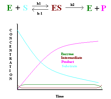
This gives the following:
\[\dfrac{d[P]}{dt} = k_2[ES] \label{6} \]
where
\[\dfrac{d[ES]}{dt} = 0 = k_1[E][S] - k_{-1}[ES] - k_2[ES] \label{7} \]
Because
\[[S] \gg [E] \label{8} \]
Using the second assumption and the fact that enzyme concentration equals the initial concentration of enzyme minus the concentration of the enzyme-substrate intermediate,
\[[E] = [E]_o - [ES] \label{9} \]
The following equation is obtained:
\[k_1[E]_o[S] = k_{-1}[ES] + k_2[ES] + k_1[ES][S] \label{10} \]
From this equation, the concentration of the ES intermediate can be found:
\[[ES] = \dfrac{k_1[E]_o[S]}{(k_{-1} + k_2) + k_1[S]} \label{11} \]
Substitute this into Equation \(\ref{6}\) gives,
\[\dfrac{d[P]}{dt} = \dfrac{k_2[E]_0[S]}{[(k_1+k_2)/k_1]+[S]} = \dfrac{k_2[E]_0[S]}{K_M+[S]} \label{12} \]
where
\[K_M = \dfrac{k_{-1}+k_{2}}{k_1} \label{13} \]
Because in most of the cases, only the initial \(d[P]/dt\) is measured to determine the rate of product formation, Equation \ref{12} can be rewritten as:
\[v_o = \dfrac{d[P]_0}{dt} = \dfrac{k_2[E]_0[S]}{K_M+[S]} \label{14} \]
Because \([E]_o = v_{max}/k_2\). Equation \(\ref{14}\) becomes the following:
\[ \begin{align} v_0 &= \dfrac{d[P]_o}{dt} \\[4pt] &= \dfrac{(k_2/k_2)v_{max}[S]}{K_M+[S]} \label{15} \\ &= \dfrac{v_{max}[S]}{K_M+[S]} \label{16} \end{align} \]
This equation is a useful tool to in calculating \(v_{max}\) and \(K_M\) (the Michaelis constant) of an enzyme by using the Lineweaver-Burk plot (1/[S] vs. 1/v0) or the Eadie-Hofstee plot (v0/[S] vs. v0).
Problems
Given the reaction \(A \xrightarrow[]{k_1} B \xrightarrow[]{k_2} C\)
where k1= 0.2 M-1s-1 , k2 = 2000 s-1
- Write the reaction rates for A, B, and C.
- Is this a steady-state reaction?
- Write the expression for d[C]/dt using the Steady State Approximation
- Calculate d[C]/dt if [A] = 1M
- Calculate [C] at t = 3 s and [A]0 = 2M
Solutions
1) d[A]/dt = -k1[A]; d[B]/dt = k1[A] - k2[B]; d[C]/dt = k2[B]
2) Because k1 is much larger than k2, this is a steady state reaction.
3) d[C]/dt = k2[B]
where d[B]/dt = k1[A] - k2[B] = 0
so, [B] = k1[A]/k2
Substitute this into d[C]/dt
d[C]/dt = k1[A]
4) d[C]/dt = 0.2M-1s-1(1M) = 0.2 s-1
5) [C] = [A]0 (1-e-k1t) = 2M(1-e-0.2(3)) = 0.9 M
References:
- Chang, Raymond. Physical Chemistry for The Biosciences. Sausalito: University Science Books, 2005. 368-370.
- Garrett, Reginald H, Charles M. Grisham. Biochemistry. 4th ed. Boston: Brooks/Cole Cengage Learning, 2010. 389-397.
- Segel, Irwin H. Biochemical Calculations. 2nd ed. New Jersey: John Wiley and Sons, inc., 1976. 216-218.
Contributors and Attributions
Chung (Peter) Chieh (Professor Emeritus, Chemistry @ University of Waterloo)
5.7: Reaction Mechanisms 2 - Steady-State Approximation is shared under a CC BY-NC-SA 4.0 license and was authored, remixed, and/or curated by LibreTexts.
The book could not be loaded just now.