Opening the book…
This textbook has been updated to a new edition and can be found here.
“Fluctuations” refers to the random or noisy time evolution of a microscopic subsystem imbedded an actively evolving environment. Randomness is a property of all chemical systems to some degree, but we will focus on an environment that is at or near thermal equilibrium. Systems at thermal equilibrium are macroscopically time-invariant; however, they are microscopically dynamic, with molecules exploring the range of microstates that are thermally accessible. Local variations in energy result in changes in molecular position, orientation, and structure, and are responsible for the activation events that allow chemical equilibria to be established.
If we wish to describe an internal variable \(A\) for a system at thermal equilibrium, we can obtain the statistics of \(A\) by performing ensemble averages described above. The resulting averages would be time-invariant. However, if we observe a member of the ensemble as a function of time, \(A_i(t)\), the behavior is generally is observed to fluctuate randomly. The fluctuations in \(A_i(t)\) vary about a mean value \(\langle A \rangle\), sampling thermally accessible values which are described by an equilibrium probability distribution function \(P(A)\). \(P(A)\) describes the potential of mean force, the free energy projected as a function of \(A\):
\[F ( A ) = - k _ {B} T \ln P ( A ) \label{8.19}\]
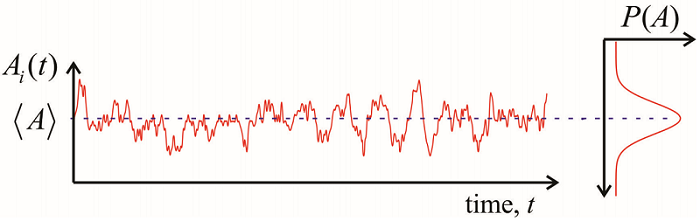
Given enough time, we expect that one molecule in a homogeneous medium will be able to sample all available configurations of the system. Moreover, a histogram of the values sampled by one molecule is expected to be equal to \(P(A)\). Such a system is referred to as ergodic. Specifically, in an ergodic system, it is possible describe the macroscopic properties either by averaging over all possible values for a given member of the ensemble, or by performing an average over the realizations of \(A\) for the entire ensemble at one point in time. That is, the statistics for \(A\) can be expressed as a time-average or an ensemble average. For an equilibrium system, the ensemble average is
\[\langle A \rangle = \operatorname {Tr} \left( \rho _ {e q} A \right) = \sum _ {n} \frac {e^{- \beta E _ {n}}} {Z} \langle n | A | n \rangle \label{8.20}\]
and the time average is \[\overline {A} = \lim _ {T \rightarrow \infty} \frac {1} {T} \int _ {0}^{T} d t \, A _ {i} (t) \label{8.21}\]
These quantities are equal for an ergodic system:
\[\langle A \rangle = \overline {A}\]
Equilibrium systems are ergodic. From Equation \ref{8.21}, we see that the term ergodic also carries a dynamical connotation. A system is ergodic if one member of the ensemble has evolved long enough to sample the equilibrium probability distribution. Experimental observations on shorter time scales view a nonequilibrium system.
This page titled 9.3: Fluctuations was last modified on Sun, 16 Aug 2026 23:52:43 GMT and is shared under a CC BY-NC-SA 4.0 license and was authored, remixed, and/or curated by Andrei Tokmakoff via source content that was edited to the style and standards of the LibreTexts platform.
The book could not be loaded just now.