Opening the book…
20.8.1 Rejection sampling
We will generate samples from our posterior distribution using a simple algorithm known as rejection sampling. The idea is that we choose a random value of x (in this case
# Compute credible intervals for example

nsamples <- 100000

# create random uniform variates for x and y
x <- runif(nsamples)
y <- runif(nsamples)

# create f(x)
fx <- dbinom(x = nResponders, size = 100, prob = x)

# accept samples where y < f(x)
accept <- which(y < fx)
accepted_samples <- x[accept]

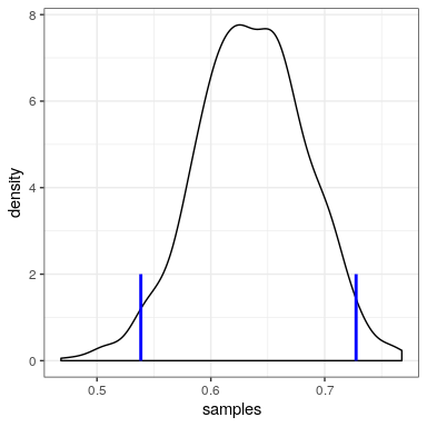
credible_interval <- quantile(x = accepted_samples,
                              probs = c(0.025, 0.975))
kable(credible_interval)| x | |
|---|---|
| 2.5% | 0.54 |
| 98% | 0.73 |
This page titled 20.8: Appendix- was last modified on Mon, 11 Jan 2021 05:14:09 GMT and is shared under a CC BY-NC 4.0 license and was authored, remixed, and/or curated by Russell A. Poldrack via source content that was edited to the style and standards of the LibreTexts platform.
The book could not be loaded just now.