Opening the book…
In this lesson, we will make inferences about the population mean difference between two quantitative measurements. We will learn how to construct interval estimates and test hypotheses using paired data.
Paired/Dependent and Independent Data
Consider the two scenarios below.
Example 1
The planet’s average surface temperature has risen about 2 degrees Fahrenheit (1 degree Celsius) since the late 19th century. Earth’s global average surface temperature in 2021 tied with 2018 as the sixth warmest year on record, according to an analysis by NASA14. In congress, there are politicians who believe that global warming is a hoax and this belief drives important policy decisions. In 2005, The New York Times reported15 that Michael Crichton, a novelist, was called to testify before the Senate Committee on Environment and Public Works. The chairman of the committee, Senator James M. Inhofe, who said that global warming is “the greatest hoax ever perpetrated on the American people,” had the committee read Crichton’s fictional novel “State of Fear” (an environmental thriller that casts doubt on the idea that human activities contribute to global warming). Crichton asserted that cooling observed in the interior of Antarctica shows the lack of reliability of models used for global warming predictions and of climate science in general. The book remains one of the most cited works in climate change skeptic circles.
Does the data in “State of Fear” disprove climate change? In the book, a graph of temperatures in Punta Arenas is shown for the last 116 years. The graph has a downward trend and suggests that the temperature is actually dropping over time. To investigate this claim, we randomly sample 32 pairs of latitudes and longitudes, find the nearest station for each set of coordinates, and measure the average temperature over two consecutive blocks of time.
Example 2
Los Angeles Daily News reported16 that “Low-income neighborhoods with higher Black, Hispanic, and Asian populations experience significantly more urban heat than wealthier and predominantly white neighborhoods in Southern California and within a vast majority of populous U.S. counties.” According to a study17, “roughly 25% of all natural hazard mortality in the U.S. is due to heat exposure (Borden & Cutter, 2008) and heat waves are becoming more frequent, more intense, and are longer in season (Shiva et al.,2019; Wobus et al., 2018); understanding who is affected by urban heating and what drives exposure disparities is therefore critical for crafting just and effective policy responses, particularly under warming climate conditions.”
A statistics student wants to know the mean difference in land surface temperature between poor and affluent communities. They randomly sample 556 counties with high rates of poverty and 500 affluent counties. They find the average temperature and sample standard deviation for each of the groups and use the sample data to estimate the population mean difference in temperature between poor and affluent communities.
Summary
- Notice any differences and similarities between the two examples.
In both examples, two sets of data were collected. In example 1, the average temperature is measured twice (from 1901-1950 and from 1951-2000) for each randomly chosen station location. In example 2, the average temperature is measured once for each group. In example 1, the two data sets are directly related in pairs. We call such data paired or dependent. A sample is paired if each subject in the sample is measured twice. In example 2, the two data sets are not directly related. The values of one set have no effect on the values of the other set. Such data is referred to as independent.
Identify Paired Samples
In the following questions, identify whether the question is solved by constructing a confidence interval or conducting a hypothesis test, and if this requires data from a paired sample or from two independent samples. Explain how you made your decision.
- Jason claims that a higher proportion of males pass their drivers test in the first attempt than the proportion of females pass the test in the first attempt.
- It is believed that the average grade on an English essay in a particular school system for females is higher than for males. A random sample of 31 females had a mean score of 82 with a standard deviation of three, and a random sample of 25 males had a mean score of 76 with a standard deviation of four. Estimate the average difference in grades for females and males.
- Eight subjects are picked at random and given a new sleep medication. The mean hours slept for each person were recorded before starting the medication and after. Estimate the mean difference in hours slept before and after use of the sleep medication.
- A new WiFi range booster is being offered to consumers. A researcher tests the native range of 12 different routers under the same conditions. The ranges are recorded. Then the researcher uses the new WiFi range booster and records the new ranges. Does the new WiFi range booster do a better job?
Construct a Confidence Interval for the Mean Difference
In example 1, we want to determine if the earth is warming. We randomly sample 32 pairs of latitudes and longitudes, find the nearest station for each set of coordinates, and measure the average temperature over two consecutive blocks of time.
- Given below is the average temperature measured from 1901-1950 and the average temperature measured from 1951-2000 for the Punta Arenas station. Does this piece of data support the claim that the earth is not warming? Use a difference to support your answer.
Nearest station
avg 1901-1950
avg 1951-2000
Difference
Punta Arenas
6.5164
6.207959184
- The difference in temperature at the Punta Arenas station is _________________ which means that the average temperature has decreased. What value for the difference would indicate that there was no change in temperature? What does this tell you about the average temperature from 1901-1950 and the average temperature from 1951-2000 at a station that has no change in temperature?
- If the difference in temperature at a station is ________________, then the average temperature has increased. Which measurement would be greater at such a station: the average temperature from 1901-1950, or the average temperature from 1951-2000? Explain why you think this.
- Given below is the data from the 32 stations in the sample. Highlight any station where the temperature decreased. For how many stations did the temperature decrease?
Nearest station
avg 1901-1950
avg 1951-2000
Difference
Tenerife Los Rodeos
14.667
15.927
1.26
Punta Arenas
6.516
6.208
-0.308
Invercargill Airport
9.239
9.784
0.545
Honolulu Intl Ap
24.292
24.486
0.194
Montevideo Prado
15.642
16.037
0.395
Eagle
-5.179
-4.359
0.82
Rarotonga Intl
23.331
23.836
0.505
Accra
26.601
26.767
0.166
Port Elizabeth Intl
17.19
17.164
-0.026
Chatham Islands
10.683
11.324
0.641
Mahe Seychellesbri
26.561
26.896
0.335
Nairobi Dagoretti
17.148
17.649
0.501
Hobart Ellerslie Road
12.299
12.818
0.519
Jask
26.545
26.372
-0.173
Manati
23.694
24.594
0.9
Cape Leeuwin
16.743
17.076
0.333
Cairns Post Office
23.726
24.647
0.921
Durban Intl
19.981
20.704
0.723
Upernavik
-7.012
-7.286
-0.274
Buenos Aires Observ
16.92
18.107
1.187
Auckland Aero Aws
14.46
15.391
0.931
Bahia Blanca Aero
14.441
14.642
0.201
Merced Muni Ap
16.236
15.94
-0.296
Albany
15.608
15.84
0.232
Concepcion
12.226
12.518
0.292
Dakar Yoff
22.727
23.569
0.842
Kazalinsk
8.242
8.912
0.67
Cherdyn
0.3
0.661
0.361
Karlstad
5.373
5.099
-0.274
Vladivostok
3.978
4.919
0.941
Rio De Janeiro
24.36
25.275
0.915
Kirensk
-4.331
-3.861
0.47
- Mark on the numberline where ‘no difference’ in temperature would be. For how many stations did the temperature warm? For how many stations did the temperature cool?

Images are created with the graphing calculator, used with permission from Desmos Studio PBC.
- At the Punta Arenas station, the temperature cooled. Do you think that this difference is representative of climate patterns across the world?
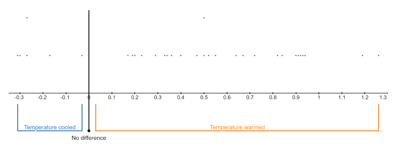
Images are created with the graphing calculator, used with permission from Desmos Studio PBC.
- Let’s estimate the mean temperature change for the earth with 95% confidence. The mean difference from our sample, \(\bar{x}=0.452\) degrees celsius, and the sample standard deviation for the differences is s=0.4361 degrees celsius.
Step 1 Is the sampling distribution approximately normal? Explain.
Step 2 Find the critical value (rounded to three decimal places) that corresponds to a ____ % confidence level and ______ degrees of freedom.
\(T_c=\operatorname{tdist}(\underline{\ \ \ \ \ \ \ \ \ \ }) \cdot \operatorname{inversecdf}(\underline{\ \ \ \ \ \ \ \ \ \ })=\underline{\ \ \ \ \ \ \ \ \ \ }\)
\(n=\underline{\ \ \ \ \ \ \ \ \ \ }\)
\(df=\underline{\ \ \ \ \ \ \ \ \ \ }\)
\(\bar{x}=\underline{\ \ \ \ \ \ \ \ \ \ }\)
\(s=\underline{\ \ \ \ \ \ \ \ \ \ }\)
Step 3 The margin of error rounded to three decimal places is
\(E=T_c \cdot \dfrac{s}{\sqrt{n}}=\underline{\ \ \ \ \ \ \ \ \ \ }\cdot\dfrac{\underline{\ \ \ \ \ \ \ \ \ \ }}{\displaystyle\sqrt{\underline{\ \ \ \ \ \ \ \ \ \ }}}=\underline{\ \ \ \ \ \ \ \ \ \ }\)
Step 4 The interval is
\((\bar{x}-E, \bar{x}+E)=(\underline{\ \ \ \ \ \ \ \ \ \ }-\underline{\ \ \ \ \ \ \ \ \ \ },\ \underline{\ \ \ \ \ \ \ \ \ \ }+\underline{\ \ \ \ \ \ \ \ \ \ })=(\underline{\ \ \ \ \ \ \ \ \ \ }, \underline{\ \ \ \ \ \ \ \ \ \ })\)
Step 5 State the conclusion in context:
Based on the interval, do you think the earth is warming or cooling? Explain.
Conduct a Hypothesis Test about the Mean Difference
Stations showed warming, on average. Is the average temperature change significantly high? Let’s test this claim at a 5% level of significance.

Images are created with the graphing calculator, used with permission from Desmos Studio PBC.
Step 1 Let \(\mu\) represent the mean global temperature change.
\(H_0: \mu=0\)
\(H_a:\underline{\ \ \ \ \ \ \ \ \ \ }\ \underline{\ \ \ \ \ \ \ \ \ \ }\ \underline{\ \ \ \ \ \ \ \ \ \ }\)
We will conduct a right-tailed test.
Step 2 Is the sampling distribution approximately normal? Explain.
\(n=\underline{\ \ \ \ \ \ \ \ \ \ }\)
\(df=\underline{\ \ \ \ \ \ \ \ \ \ }\)
\(\bar{x}=\underline{\ \ \ \ \ \ \ \ \ \ }\)
\(s=\underline{\ \ \ \ \ \ \ \ \ \ }\)
Step 3 Compute the test statistic rounded to three decimal places. Use it to compute the P-value.
\(T=\dfrac{\bar{x}-\mu}{\dfrac{s}{\sqrt{n}}}=\dfrac{\underline{\ \ \ \ \ \ \ \ \ \ }}{\dfrac{\underline{\ \ \ \ \ \ \ \ \ \ }}{\sqrt{\underline{\ \ \ \ \ \ \ \ \ \ }}}}=\underline{\ \ \ \ \ \ \ \ \ \ }\)
P-value is ______________
Step 4 State the conclusion in context:
Reference
14Climate Change: Vital Signs of the Planet. 2022. Climate Change Evidence: How Do We Know? accessed June 28 2022, https://climate.nasa.gov/evidence/
15 “Michael Crichton, Novelist, Becomes Senate Witness,” Michael K Janofsky, Sept 29, 2005, accessed June 28, 2022, https://www.nytimes.com/2005/09/29/books/michael-crichton-novelist-becomes-senate-witness.html
16“Poor neighborhoods get up to 7° hotter than rich ones in Southern California, study finds,” July 13, 2021, accessed June 28, 2022, https://www.dailynews.com/2021/07/13/poor-southern-california-communities-suffer-more-from-extreme-heat-ucsd-study-finds/
17“Widespread Race and Class Disparities in Surface Urban Heat Extremes Across the United States,” Susanne Amelie Benz and Jennifer Anne Burney, July 13, 2021, accessed June 28, 2022, https://agupubs.onlinelibrary.wiley.com/doi/10.1029/2021EF002016
This page titled 8.1: Paired Samples was last modified on Thu, 20 Feb 2025 19:17:41 GMT and is shared under a CC BY-NC-SA 4.0 license and was authored, remixed, and/or curated by Hannah Seidler-Wright.
The book could not be loaded just now.