Opening the book…
Our first step in assessing the effectiveness of our artifact correction+rejection pipeline is to determine whether blinks are a confound, meaning that they differ across the conditions we will be comparing. If they differ across conditions, then they could create a bogus experimental effect or distort the time course or scalp distribution of a real effect. When blinks are a confound and not just a source of noise, this increases the stakes for having an effective correction+rejection pipeline.
We have mainly focused on the MMN paradigm so far in our chapters on artifact rejection and correction, and given that the stimuli in this paradigm were task-irrelevant, it is unlikely that blinks would differ between deviants and standards. Indeed, Zhang et al. (2024) found that the blinks were random with respect to the stimuli in this paradigm. Consequently, the remainder of this chapter will focus on the N400 paradigm, which has some very interesting blink patterns that will demonstrate what you should look for in your own studies.
As a reminder, each trial in this paradigm consisted of a prime word followed by a target word, and the target word was either semantically related to or unrelated to the prime word. The task was to press one of two buttons following each target to indicate whether it was related or unrelated to the preceding prime. The N400 component was much larger (more negative) for unrelated targets than for related targets. The N400 was measured as the mean amplitude from 300-500 ms in the unrelated-minus-related difference wave at the CPz electrode site. The details are presented in Sections 2.2 and 2.3 of Chapter 2.
General Approach
Our question in this exercise is whether blinks differed between related and unrelated targets. There is no obvious reason to expect a difference, but it is important to test for a difference rather than assuming the lack of a difference. One thing my lab learned when we carefully examined the artifacts in the ERP CORE paradigms (Zhang et al., 2024) is that blinks often differed between conditions in ways that we did not expect.
Note that we will focus on blinks in this exercise and largely ignore eye movements, which were rare in the N400 paradigm. Participants were motivated to keep their gaze on the central fixation point in this paradigm, and we saw zero eye movements during the task in most participants. In addition, the ICA decomposition did not yield a clear eye movement IC for most participants.
We are going to examine differences in blinking between conditions in two ways. First, we will apply artifact detection to the uncorrected VEOG-bipolar channel and count how many trials in each condition were marked for rejection. Second, we will ask whether the time course of the blinks differed between conditions by comparing the waveforms for related targets and unrelated targets in the uncorrected VEOG-bipolar channel in the averaged ERPs.
If you looked at this information in the data from a single participant, you wouldn’t know whether any differences were random or systematic. To assess whether there are systematic differences in blinking between conditions, you need to look at the data from all the participants. This would take a very long time in the eStudio GUI, so I wrote some Matlab scripts that prepared the data for you.
I limited the analyses to 20 of the 40 participants to keep things simple (and, if I'm being honest, to save myself some time). I first limited the analyses to the 10 participants that were analyzed in Chapter 3. I then realized that I had originally chosen those 10 participants because they had beautiful data, so they weren’t very good for demonstrating artifact correction and detection. I therefore added another 10 participants who had more typical data. It’s still not a random sample of the 40 participants who were included in the original ERP CORE study (Kappenman et al., 2021), so the results you will see here will not quite match what was reported by Zhang et al. (2024). However, the general pattern is the same.
The Data
You can find the N400 data in a folder cleverly named N400_Data inside the Chapter_9 folder. The initial EEGsets in this folder have already been preprocessed a little, including high-pass filtering the data at 0.1 Hz, referencing the EEG and EOG channels to the average of P9 and P10, and creating bipolar VEOG and HEOG channels. Each of these EEGsets is named X_N400_preprocessed.set, where X is the subject number. The folder also contains three scripts that implemented ICA-based artifact correction for these 20 participants following the recommendations in Section 9.7:
- N400_correction_rejection_phase1.m took each participant’s initial EEGset (X_N400_preprocessed) and made a copy of this EEGset (named X_N400_preprocessed_optimized) that was optimized for the ICA decomposition process. This involved downsampling to 100 Hz, filtering from 1-30 Hz, deleting break periods, and deleting any segments of the continuous data that contained extra-huge C.R.A.P. that might interfere with the ICA decomposition.
- N400_correction_rejection_phase2.m took each participant’s optimized EEGset and performed the ICA decomposition (excluding the bipolar EOG channels and any “bad” channels that would later be interpolated). This resulted in an EEGset for each participant named X_N400_preprocessed_optimized_weights.
- N400_correction_rejection_phase3.m transferred the ICA weights back to the original EEGset and then used those weights to perform the artifact correction by reconstructing the EEG from the ICs, but without the ICs corresponding to blinks and possibly eye movements (if a clear eye movement IC was present). Interpolation was then performed on the “bad” channels. The resulting EEGset was named X_N400_preprocessed_pruned.
These scripts made use of Excel files that I created to store information about which channels were bad, what parameters should be used to reject huge C.R.A.P. from each participant’s continuous EEG data, and which ICs corresponded to blinks and eye movements and should therefore be removed. The output files of these scripts are available in the N400_Data folder, so you do not need to run the scripts. However, you will find them very useful as models for writing scripts to apply this approach to your own data.
Counting the Number of Blinks Per Condition
To count the number of blinks per condition for each participant, I created and ran a script named N400_correction_rejection_phase4_count_blinks.m.
Statistics Toolbox
The script N400_correction_rejection_phase4_count_blinks.m uses the Matlab ttest() function, which is part of the Statistics and Machine Learning Toolbox. You can see what toolboxes are installed by typing ver on the Matlab command line. If you do not have this toolbox, I recommend consulting your IT department to see if you can get it for free as a part of your license. You can also purchase it from The Mathworks.
If you cannot get this toolbox, the script has information about how to comment out the lines that use the ttest() function.
For each of our 20 participants, this script took the ICA-corrected data (X_N400_preprocessed_pruned), added an EventList, ran BINLISTER using a bin descriptor file named BDF_N400_Targets.txt to sort the events into bins (bin 1 = related targets; bin 2 = unrelated targets), and epoched the data. Then, artifact detection was applied to the uncorrected VEOG-bipolar channel to mark epochs containing blinks. I used the moving window peak-to-peak amplitude algorithm with a threshold of 100 µV, looking for blinks in every 200-ms window within the 1000-ms epoch. I checked to make sure that this threshold worked well for each of the 20 participants. The resulting EEGset was saved in a file named X_N400_preprocessed_pruned_be_allblinksmarked.set. Keep in mind that these epochs were marked solely to determine if the number of blinks differed between conditions; these blinks have already been corrected in the EEG channels via ICA, but we want to know if they are a confound and whether ICA eliminated this confound.
Using these EEGsets, the script created an averaged ERP for each participant. I included this step because it’s really easy to get a count of the number of artifacts in each bin from an ERPset. This information could be derived from the EventList in the EEGsets, but it’s a lot easier to see it in an ERPset.
To see the results of this set of steps, first reset everything with the Reset button. Then change the current folder to N400_Data using the Current Folder button in the EEGsets panel, and then load the EEGset for Subject 1 with the blinks marked (1_N400_preprocessed_pruned_be_allblinksmarked.set). Start scrolling through the EEG, looking for epochs that have been marked for rejection because of blinks in the VEOG-bipolar channel (which was excluded from the ICA decomposition and the subsequent artifact correction). You’ll see no blinks in the first 30 epochs. Then you’ll see that blinks started occurring more often. This is a common pattern; many participants initially suppress their blinking because they are focusing on the task, but then their eyes start to dry out, and they start blinking.
Because we planned to apply artifact correction to these data, the only instruction we gave participants was to avoid blinking prior to making their buttonpress response on each trial. As a result, there were lots of blinks, mainly after the response at ~400 ms. You can see that most of Subject 1’s blinks were in the second half of the epoch.
Now go to the Artifact Info & Tools panel and click Artifact Summary. A window should appear with the table shown in Screenshot 9.22. You can see that 31.82% of epochs were marked as containing blinks, with 19 marked epochs for bin 1 (related targets) and 16 marked epochs for bin 2 (unrelated targets).

Screenshot 9.22
Although it’s easy to view the number of marked epochs per bin in an EEGset using the eStudio GUI, this information is a little more difficult to extract using a script. The script therefore used this EEGset to create averaged ERPs, with the ERPset named 1_N400_count_blinks.erp. Go to the ERP tab and load this ERPset using the ERPsets panel.
If you go to the ERP & Bin Information panel, you can again see that 19 epochs were marked for rejection in bin 1 and 16 epochs were marked in bin 2. You can also get this information by going to the Command Window and typing ERP.ntrials. You should see something like Screenshot 9.23. This shows the number of accepted and rejected trials for each bin. This information is directly accessible by a script.
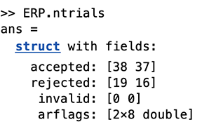
Screenshot 9.23
If you do a little arithmetic with these numbers, you can determine that 33.3% of trials were marked for blinks in bin 1 (related targets) and 30.2% of trials were marked in bin 2 (unrelated targets). Is that small difference just noise, or is it a consistent difference between related and unrelated targets? To answer that question, we will need to look at all of the participants.
To avoid doing a lot of arithmetic by hand, I had the script calculate these proportions for each participant, store them in an Excel spreadsheet named Blinkrate.xslx, and display the mean across participants for each bin along with a statistical test of the difference between the two bins. These values are shown in the Command Window, like this:
Blink rate for related targets: 0.439
Blink rate for unrelated targets: 0.351
t(19) = 2.93, p = 0.0086
You can see that, across the 20 participants included in this analysis, people blinked about 9% more following related targets than following unrelated targets, and that this was a statistically significant difference. I have no idea why people blinked more in response to the related targets, and I don’t really care, because I am not a psycholinguist. However, I do care that there was a consistent difference in blinking between related and unrelated targets, because this is a confound. If we do not deal with the voltages produced by these blinks, they will create an artifactual difference between the ERPs for related and unrelated targets.
Note that you can see the spreadsheet with the single-participant values (Blinkrate.xslx) by going back to the Chapter_9 folder. You can run the script by going to the Chapter_9 folder and typing N400_correction_rejection_phase4_count_blinks in the Command Window.
Comparing the Blink Waveforms for the Two Conditions
In addition to counting the number of blinks in each condition, it’s also important to examine the uncorrected VEOG-bipolar waveforms for the two conditions. Even if the number of blinks is the same across conditions, the timing might be different, and that could lead to differences in blink voltages between the two conditions at some time points. Indeed, when my lab looked at the error-related negativity data from the ERP CORE, we found that the number of blinks was nearly identical for error trials and correct trials, but the blinks were later for the error trials than for the correct trials (Zhang et al., 2024).
To avoid being fooled by idiosyncratic single-participant results, it’s best to compare the blink waveforms using grand average ERP waveforms. To see this for the N400 experiment, make sure that the Chapter_9 folder is Matlab’s current folder, click the Load ERP button in the ERPsets panel, and select Grand_N400_no_correction_or_rejection.erp. This grand average was created with a script named N400_correction_rejection_phase4_baseline.m, which I will describe in more detail in the next section. No artifact correction or rejection was applied in the pipeline that produced this ERPset.
Select only channel 33 (VEOG-bipolar) in the Bin & Channel Selection panel and click Apply; this will show you only the uncorrected bipolar VEOG signal. It should look something like Screenshot 9.24. You can see that the blink waveform is substantially larger (more negative) for the related targets than for the unrelated targets. The blink voltage also appears to start earlier for the related targets, and there is a substantial difference in voltage between related and unrelated targets in the N400 measurement window (300-500 ms). Uh oh! We need to make sure that our artifact correction procedure actually eliminated this confound.

Screenshot 9.24
Now go back to the Bin & Channel Selection panel, select All channels, and click Apply. If you look at the VEOG-lower channel (which is the electrode under the left eye referenced to the average of P9 and P10), you will see that the voltage is more negative for unrelated targets than for related targets, just as we saw in the VEOG-bipolar channel. Blinks are negative under the eye, so this greater negative voltage for related targets is consistent with our earlier data showing that blinks were more common for related targets than for unrelated targets.
If you look at FP1 and FP2, you’ll see that the voltage is more positive for related targets than for unrelated targets. Blinks are positive at FP1 and FP2, so this is also likely a result of the greater number of blinks for related targets. This difference between related and unrelated targets is smaller at the F3, Fz, and F4 electrodes, which makes sense given that the amplitude of a blink falls off as we move away from the eyes.
If you look at CPz, you’ll see that the voltage is also more positive for related targets than for unrelated targets. But we could rephrase this as the voltage being more negative for unrelated targets than for related targets, which is the usual way of describing the usual N400 effect. So, is the effect at CPz the N400 effect, or is it just the difference in voltage we see as a resulting of blinking at FP1 and FP2, volume-conducted from the eyes back to CPz?
Yikes! These findings raise the possibility that the venerable N400 effect, which has been observed in hundreds of published studies, might be a blink artifact rather than reflecting differences in brain activity for related and unrelated targets. But keep in mind that we haven’t done any correction or rejection for blinks, and almost all N400 studies have at least attempted to minimize blink activity. So, the N400 effect in this experiment is probably safe. But to be sure, we need to determine whether our artifact correction+rejection procedure has done a good job of reducing the blink-related activity. This shows the importance of evaluating the effectiveness of your pipeline for dealing with artifacts. If it’s not effective, your effects may reflect blink artifacts instead of brain activity (or a mixture of artifacts and brain activity).
This page titled 9.9: Exercise- Determining Whether Blinking is a Confound was last modified on Thu, 01 Oct 2026 18:52:30 GMT and is shared under a CC BY-NC 4.0 license and was authored, remixed, and/or curated by Steven J Luck.
The book could not be loaded just now.