12.4: Exercise- Binary Decoding of ID 1 versus ID 2

In our first exercise, we're going to do a simple binary decoding of ID 1 versus ID 2 for one participant in the study of Bae (2021). But first let’s take a look at the EEG and event codes and do some preprocessing.

Reset everything with the Reset button and set the Current Folder to the Chapter_12 folder. In the EEG tab, click Load EEG in the EEGsets panel, navigate to Bae_Data > 302, and select the file named 302_preprocessed.set. The first subject, 301, had a few extra event codes, so we’re going to focus on the data from Subject 302 in this exercise. We'll look at the data from Subject 301 later.

Now scroll through the data from 302_preprocessed as you normally would when beginning to process a file.

All channels in this EEGset have been referenced to the average of the left and right mastoids, and the data have been filtered from 0.1–20 Hz. An EventList has been added. ICA has already been applied to this EEGset to correct blinks and eye movements. The EOG channels have not been corrected, so you will see blinks only in the VEOG L channel (VEOG-lower referenced to average mastoids) and the VEOG L-U channel (VEOG-lower minus Fp2), which were not corrected. You’ll also see eye movements only in the HEOG L and HEOG R channels (HEOG-left and -right referenced to average mastoids) and the HEOG R-L channel (HEOG-right minus HEOG-left), which were also left uncorrected. We will exclude these uncorrected channels from the decoding process.

If you scroll far enough, you’ll start seeing event codes. Here are the event codes for the 16 different combinations of face ID and emotional expression:

Event codes for the 16 different combinations of face ID and emotional expression

	Fearful	Happy	Neutral	Angry
ID 1	211	221	231	241
ID 2	212	222	232	242
ID 3	213	223	233	243
ID 4	214	224	234	244

ERPLAB uses its standard bin approach to define the classes for decoding. To decode a set of classes, you start by using BINLISTER to assign each event to the appropriate bin for each class. If you double-click on BDF_ID_Expression.txt in Matlab’s Current Folder pane, you can see that 8 bins have been defined. Bins 1 through 4 correspond to ID 1 through ID 4, including all four emotional expressions for each ID. For example, Bin 1 corresponds to ID 1 and includes event codes 211, 221, 231, and 241. Bins 5-8 correspond to the four emotional expressions, including all four IDs in the bin for a given expression. When I decoded face identity (Figure 12.1), I did this by telling ERPLAB to use Bins 1-4 to define the four classes. When I decoded emotion expression, I told ERPLAB to use Bins 5-8 to define the four classes.

Now that you’ve seen how the bins are defined, let’s run BINLISTER with this set of bin definitions. Go to the Assign Events to Bins panel, click the Browse button, and select the file named BDF_ID_Expression.txt. Then click Run and use the default EEGset name (302_preprocessed_bins). The panel will show you that there are 160 occurrences of each of the 8 bins. There were 40 trials for each of the 16 ID/emotion combinations, so this gives us 160 trials for each ID (collapsed across emotions) and 160 trials for each emotion (collapsed across IDs).

The next step is to epoch the data. Go to the Extract Bin-Based Epochs panel, make sure the epoch is set to -200 800 and that the baseline period is set to Pre, and click Apply. When the naming/saving window appears, use the default EEGset name (302_preprocessed_bins_be). Click Run. In the main eStudio plotting region, you should see that you now have epochs of 200-800 ms for each trial, with each epoch labeled with one of the eight bins.

We’re now ready to begin the specific steps needed for decoding. The first step is to convert this EEGset into something called a bin-epoched single-trial set (BESTset). A BESTset contains bin-epoched data in a super-efficient organization. Each bin is stored as a 3-dimensional matrix of channels x time points x trials. We designed this data structure for decoding, but if you ever write custom scripts to apply some kind of new algorithm to single-trial EEG epochs, this format could be very useful. 

To convert the current EEGset into a BESTset, make sure that 302_preprocessed_bins_be is still selected in the EEGsets panel, and go to the panel named Extract Bin-Epoched Single Trials. The option labeled Only epochs without flagged artifacts should be set (so that epochs flagged with artifacts are excluded), as should the option for Exclude epochs with boundary events. Although we’re only going to decode ID 1 and ID 2 (bins 1 and 2) in this exercise, make sure that all 8 bins are selected (so we can use the same BESTset for later exercises). Do not check the box labeled Transform into phase-independent power; this option allows you to decode on the basis of the power in a given frequency band, which we will do in a later exercise. Click Run, change the name of the BESTset to 302, check the boxes for Save BESTsets to disk and Use bestname as filename, and click Okay.

After a moment, you'll be automatically taken out of the EEG tab and into the Pattern Classification tab. This is where the magic happens! You should see that the BESTset you just created, named 302, is in the BESTsets panel. This panel is analogous to the EEGsets and ERPsets panels, with options for loading, renaming, saving, and clearing BESTsets. Note that nothing is plotted when a BESTset is loaded. The plotting area in the Pattern Classification tab is used for plotting decoding accuracy, as we will see soon.

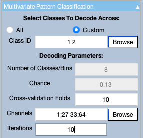
Make sure that 302 is selected in the BESTsets panel, and then go to the Multivariate Pattern Classification panel. This is a large and complicated panel, but we’ll walk through it bit by bit. The first step is to select the classes used for decoding. By default, it will decode among all of the bins, so All is probably set. We want to decode only ID 1 versus ID 2 (bins 1 and 2), so click the Custom button and enter 1 2 in the Class ID text box (and press the Tab key to make sure that your choice was entered).

Now let’s set up the Decoding Parameters section of the panel. The Number of Classes/Bins field should be set to 2 because you entered 2 bins in the Class ID field. The Chance value should therefore be set to 0.5 (1 out of 2). You can’t control these parameters directly; they are determined by the number of classes/bins you selected in the Class ID field. 

A value that you can select is the number of Cross-validation Folds. This determines what N to use for the N-fold cross-validation procedures. It also indirectly determines the number of trials that will be averaged together for each pseudotrial, which is the total number of available trials per class divided by the number of folds. Set this value to 10. Set the channels panel to 1:27 33:64, which will select just the EEG channels (and exclude the mastoid and EOG channels). Finally, set the number of Iterations to 10. We usually use more than 10 iterations, but that can make the decoding process very slow, so we’ll keep it at 10 for these exercises. The top portion of the panel should now look like Screenshot 12.1. 

Now go to the Number of trials and averages section and select the options for Equal Trials, Equal AVGs and Across Classes (and don't check the box for Across BESTsets, which I will explain later).

Now click the button labeled Show summary of trials and averages near the bottom of the panel. It will pop up a window like the one shown in Screenshot 12.2, summarizing which bins have been selected as the classes for decoding. You can see that Class 1 is Face ID 1 and Class 2 is Face ID 2. You can also see that there are 160 trials available for each of these bins (the N(trials) column), that the number of pseudotrials/averages per bin is set to 10 (the B(ERPs) column), and that each ERP (pseudotrial) will be the average of 16 trials (the N(per ERP) column). With 160 trials and 10 pseudotrials/averages per bin (which is the same as the number of folds), we automatically get 16 trials per average.

Close this summary window and look at the options near the bottom of the Multivariate Pattern Classification panel to make sure that Metric is set to ACC and that Normalization and Temporal generalization matrix are set to Off. I will explain these options later. 

Now click the Options button near the bottom of the panel, which will pop up a new window, and set everything in that window to match Screenshot 12.3. Make sure that the Algorithm is set to SVM with a Regularization value of 1 and One vs All coding. [See Zhang et al. (2026) if you want to know more about the regularization parameter and why 1 is a good value.]

I recommend setting Parallelization to Yes if your computer has a multicore processor with at least 8 cores. Decoding can take a very long time to run, but it can easily run in parallel across multiple processing cores. If you have a multicore processor, turning on the parallelization can make the decoding run much, much faster. Note that the decoding routine leaves one core unused so that you can still do other things while the decoding is running.

For the exercises in this chapter, we are also going to check the Downsample box and set the Decode every T (ms) value to 20. Rather than decoding at every time point (every 4 ms with this dataset), this option sets it to decode every 5th time point (every 20 ms). This will allow it to run in 1/5 the amount of time required to decode every single time point. In my lab, we typically run our preliminary decoding analyses with this downsampling to make the decoding run faster. Once we’ve finalized the analysis pipeline, we set it to decode every time point (and then let it run overnight or even for a couple days).

Once you have everything set, click Okay to go back to the main decoding panel, and then click Run to actually perform the decoding. A window will appear that allows you to name the output. The output of the decoding process is called a multivariate pattern classification set or MVPCset. You can use the default name (which is simply 302).

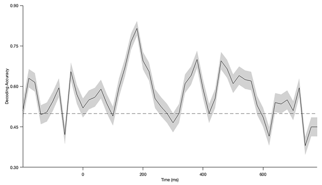
It will take some time for the decoding to finish running (somewhere between 15 seconds and 10 minutes). Nothing will seem to happen at first, because it takes some time for Matlab to get the parallel processing running. Then you will see some messages along the bottom of the eStudio window showing which iteration is running. When it is done, the new MVPCset will appear in the MVPCsets panel, and you should see a decoding waveform like that shown in Screenshot 12.4. It won’t look exactly the same, however, because the trials are randomly assigned to the pseudotrials, and this creates some variability in the decoding. That variability will be small if you run a lot of iterations, but we are only running 10 iterations here, so the results will vary a bit each time you run the decoding. [You can prevent this by doing the decoding from a script and setting the seed of the random number generator to the same value each time the script runs.]

The first thing to note about the decoding waveform is that the chance level (0.5) is shown as a dashed line. Decoding accuracy should hover around this value during the prestimulus interval. If the decoding is consistently above or below chance during the prestimulus interval, that almost always indicates that there is a problem with the decoding or the experimental design. In Screenshot 12.4, you can see that the values bounce up and down around the chance line until approximately 100 ms. At this point, the neural signal contains some information that can distinguish between ID 1 and ID 2, and decoding accuracy rises quickly. However, this is a single participant, and there is still a lot of noise, so we shouldn’t try to interpret the variations in decoding accuracy between 100 and 800 ms.

You’ve done it! You’ve taken the EEG data from a single participant and decoded whether the participant was viewing ID 1 or ID 2 at each time point. Spend a moment considering how amazing this is. The data were recorded from electrodes on the skin, a long distance from the parts of the brain involved in face processing, and yet we can decode which of two faces the participant was viewing. And we can do this separately at each moment in time. In my view, this is a minor miracle! I never would have thought this was possible 10 years ago. Not only is it possible, but it’s also pretty easy to do with ERPLAB Studio.

Of course, there are some limitations to this decoding. The first is that we decoded from averages of 16 trials, not from individual trials. Single-trial decoding is possible when the classes being decoded produce very different patterns of voltage on the scalp, but it does not usually work well for subtle classifications like different faces. Another limitation is that the decoding accuracy is far from perfect. The decoding of ID 1 versus ID 2 is far too low to be used for engineering applications such as brain-computer interfaces. However, it is good enough for answering a lot of interesting scientific questions (see Hebart & Baker, 2018, for an excellent discussion of the differing needs of scientific versus engineering applications of decoding).

---