Opening the book…
Now let’s make averaged ERPs for the bins we created. We still have continuous EEG data, so we first need to extract fixed-length epochs from the data, with the time-locking event code as time zero. Make sure that the final EEGset from the previous exercise is selected in the EEGsets panel (12_P3_corrected_elist_bins), and then go to the Extract bin-based epochs panel. Use the default epoch of -200 800 and select Pre as the baseline period (which will use the prestimulus interval). Click Apply and keep the suggested name of 12_P3_corrected_elist_bins_be for the new dataset.
When you do this, two very noticeable things will happen. First, different panels will now be grayed out, because some panels operate only on epoched data and other panels operate only on continuous data. Second, the plotting region of the eStudio GUI will show 5 distinct data epochs instead of a single continuous set of waveforms (see Screenshot 6.4). Take a look at the epoched EEG data to make sure everything looks okay.

Screenshot 6.4
Now let's make averaged ERPs from these EEG epochs using the Compute averaged ERPs panel. You should be able to use the default settings and just click RUN. You'll then see the usual panel for naming and saving the resulting ERPset. Name it 12_P3, and click the Save ERPsets to disk and Use ERP name as filename boxes so that the file will be named 12_P3.erp.
Two things will then happen. First, the main eStudio GUI will switch from the EEG tab to the ERP tab, with 12_P3 in the ERPsets panel. Second, a window will appear summarizing the results of the averaging process, as shown in Screenshot 6.5. This window allows you to verify that the expected number of trials was averaged in each bin. It also provides a summary of the aSME metric of data quality. We'll say more about that later in this chapter.
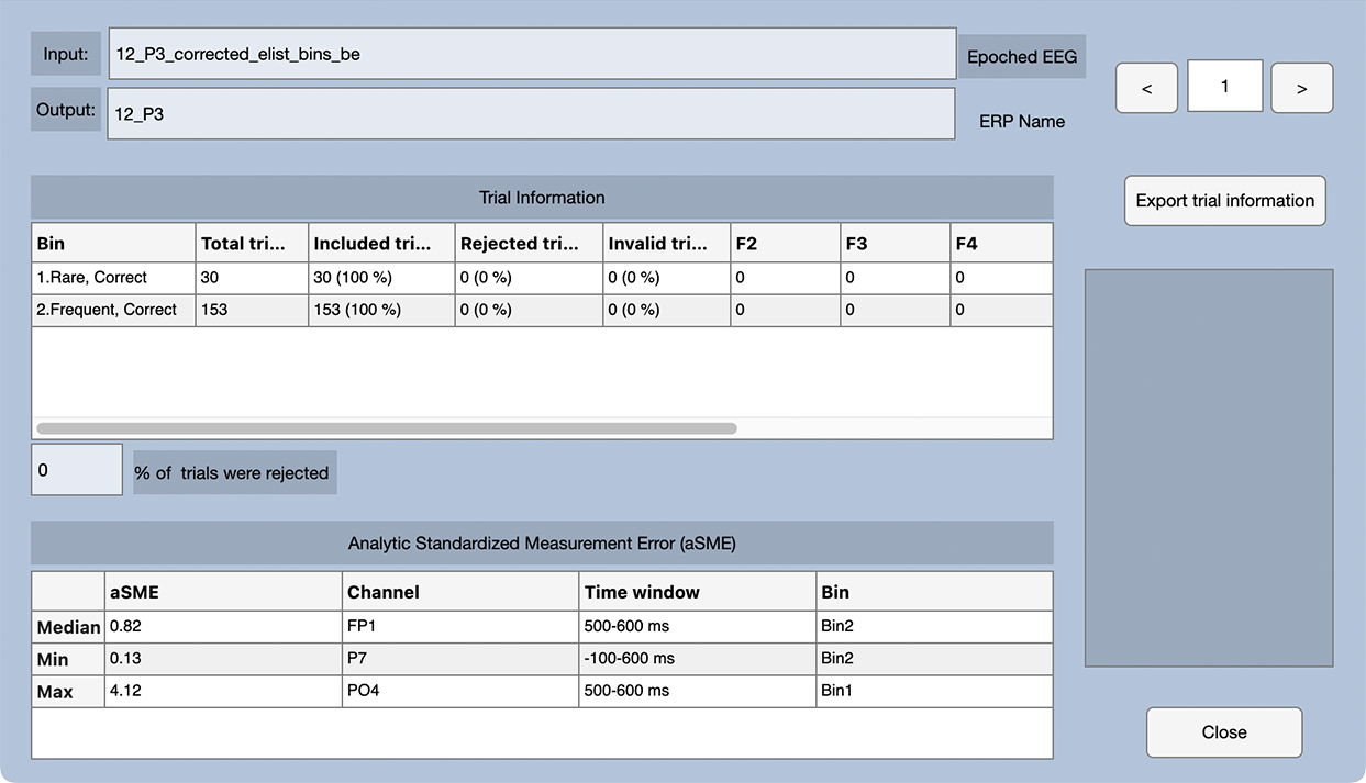
Screenshot 6.5
You can close that window and take a look at the averaged ERPs in the main eStudio GUI. To get a layout that better matches the scalp locations of the electrodes, go to the Plot Settings panel, change the Grid Layout to Custom, click the Import button, select the file named GridLocations_CustomP3b.tsv, and then click the Apply button. I've created the grid locations file for you, but you can read how to do it yourself in the ERPLAB Studio documentation.
You should now see something like Screenshot 6.6. It's a beautiful effect, with a larger P3b for the rare stimuli than for the frequent stimuli, with a maximum difference between conditions at the midline central and parietal sites.
Screenshot 6.6

But note that I intentionally chose a participant with beautiful prototypical effects for the exercises in this chapter. There are tremendous individual differences in ERP waveforms (largely due to nonfunctional differences in biophysical factors like skull thickness), and the ERPs for most of the participants in this study don’t look this much like the grand average. Averaging (whether across trials or across participants) is often necessary, but the result is something of a fiction. As I like to say, “averaging hides a multitude of sins.”
Although published papers often focus on just a few electrode sites, you should always look at the whole set of channels to verify that the scalp distribution is sensible. With a reference at or near the mastoids, the P3b effect (defined as the difference between Rare and Frequent) should be biggest along the midline near Cz and Pz. This participant’s P3b is a little more frontal than is typical for a visual paradigm, and I would ordinarily expect a smaller effect at Fz and a larger effect at Oz. But given the large range of individual differences in ERPs, this participant’s data look pretty normal.
You can also see quite a bit of high-frequency noise in the frontal and central channels over the right hemisphere (especially F8). The noise in F8 and surrounding channels is probably EMG from the temporalis muscle (the muscle near the temples that is used to contract the jaws). If you scroll through the original EEG data, you can also see the high-frequency noise in the single trials. My guess is that this participant was clenching their jaw just a little bit, mainly on the right side.
This page titled 6.6: Exercise - Looking at the Averaged ERPs was last modified on Thu, 01 Oct 2026 18:52:55 GMT and is shared under a CC BY-NC 4.0 license and was authored, remixed, and/or curated by Steven J Luck directly on the LibreTexts platform.
The book could not be loaded just now.