5.3: Graphical Interpretation and Properties of the Definite Integral

Evaluating Definite Integrals

Evaluating definite integrals this way can be quite tedious because of the complexity of the calculations. Later in this chapter we develop techniques for evaluating definite integrals without taking limits of Riemann sums. However, for now, we can rely on the fact that definite integrals represent the area under the curve, and we can evaluate definite integrals by using geometric formulas to calculate that area. We do this to confirm that definite integrals do, indeed, represent areas, so we can then discuss what to do in the case of a curve of a function dropping below the \(x\)-axis.

Example \(\PageIndex{1}\): Using Geometric Formulas to Calculate Definite Integrals

Use the formula for the area of a circle to evaluate \(\displaystyle ∫^6_3\sqrt{9−(x−3)^2}\,dx\).

Solution

The function describes a semicircle with radius 3. To find

\[∫^6_3\sqrt{9−(x−3)^2}\,dx \nonumber \]

we want to find the area under the curve over the interval \([3,6].\) The formula for the area of a circle is \(A=πr^2\). The area of a semicircle is just one-half the area of a circle, or \(A=\dfrac{1}{2}πr^2\). The shaded area in Figure \(\PageIndex{1}\) covers one-half of the semicircle, or \(A=\dfrac{1}{4}πr^2\). Thus,

\[∫^6_3\sqrt{9−(x−3)^2}\,dx=\dfrac{1}{4}π(3)^2=\dfrac{9}{4}π≈7.069. \nonumber \]

Area and the Definite Integral

When we defined the definite integral, we lifted the requirement that \(f(x)\) be nonnegative. But how do we interpret “the area under the curve” when \(f(x)\) is negative?

Net Signed Area

Let us return to the Riemann sum. Consider, for example, the function \(f(x)=2−2x^2\) (shown in Figure \(\PageIndex{2}\)) on the interval \([0,2]\). Use \(n=8\) and choose {\(x^∗_i\)} as the left endpoint of each interval. Construct a rectangle on each subinterval of height \(f(x^∗_i)\) and width \(Δx\). When \(f(x^∗_i)\) is positive, the product \(f(x^∗_i)Δx\) represents the area of the rectangle, as before. When \(f(x^∗_i)\) is negative, however, the product \(f(x^∗_i)Δx\) represents the negative of the area of the rectangle. The Riemann sum then becomes

\[\sum_{i=1}^8f(x^∗_i)Δx= (\text{Area of rectangles above the }x\text{-axis})−(\text{Area of rectangles below the }x\text{-axis}) \nonumber \]

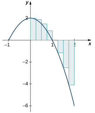
Taking the limit as \(n→∞,\) the Riemann sum approaches the area between the curve above the \(x\)-axis and the \(x\)-axis, less the area between the curve below the \(x\)-axis and the \(x\)-axis, as shown in Figure \(\PageIndex{3}\). Then,

\[\int^2_0f(x)\,dx=\lim_{n→∞}\sum_{i=1}^nf(c_i)Δx=A_1−A_2. \nonumber \]

The quantity \(A_1−A_2\) is called the net signed area.

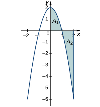
Notice that net signed area can be positive, negative, or zero. If the area above the \(x\)-axis is larger, the net signed area is positive. If the area below the \(x\)-axis is larger, the net signed area is negative. If the areas above and below the \(x\)-axis are equal, the net signed area is zero.

Example \(\PageIndex{2}\): Finding the Net Signed Area

Find the net signed area between the curve of the function \(f(x)=2x\) and the \(x\)-axis over the interval \([−3,3].\)

Solution

The function produces a straight line that forms two triangles: one from \(x=−3\) to \(x=0\) and the other from \(x=0\) to \(x=3\) (Figure \(\PageIndex{4}\)). Using the geometric formula for the area of a triangle, \(A=\dfrac{1}{2}bh\), the area of triangle \(A_1\), above the axis, is

\(A_1=\dfrac{1}{2}3(6)=9\),

where \(3\) is the base and \(2(3)=6\) is the height. The area of triangle \(A_2\), below the axis, is

\(A_2=\dfrac{1}{2}(3)(6)=9,\)

where \(3\) is the base and \(6\) is the height. Thus, the net area is

\(\displaystyle ∫^3_{−3}2x\,dx=A_1−A_2=9−9=0.\)

Analysis

If \(A_1\) is the area above the \(x\)-axis and \(A_2\) is the area below the \(x\)-axis, then the net area is \(A_1−A_2\). Since the areas of the two triangles are equal, the net area is zero.

Exercise \(\PageIndex{2}\)

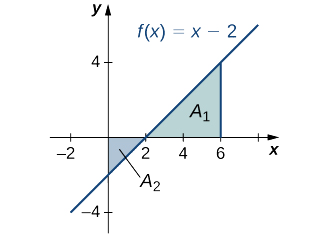
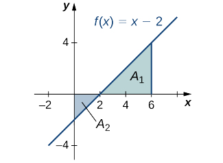
Find the net signed area of \(f(x)=x−2\) over the interval \([0,6]\), illustrated in the following image.

Hint

Use the solving method described in Example \(\PageIndex{3}\).

Answer

6

Total Area

One application of the definite integral is finding displacement when given a velocity function. If \(v(t)\) represents the velocity of an object as a function of time, then the area under the curve tells us how far the object is from its original position. This is a very important application of the definite integral, and we examine it in more detail later in the chapter. For now, we’re just going to look at some basics to get a feel for how this works by studying constant velocities.

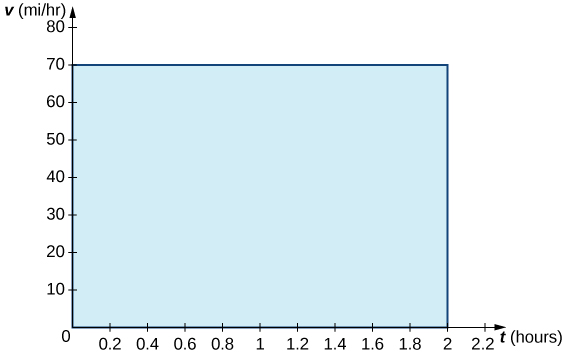
When velocity is a constant, the area under the curve is just velocity times time. This idea is already very familiar. If a car travels away from its starting position in a straight line at a speed of \(70\) mph for \(2\) hours, then it is \(140\) miles away from its original position (Figure \(\PageIndex{5}\)). Using integral notation, we have

\[∫^2_0 70\,dt=140 \,\text{miles}. \nonumber \]

In the context of displacement, net signed area allows us to take direction into account. If a car travels straight north at a speed of 60 mph for 2 hours, it is 120 miles north of its starting position. If the car then turns around and travels south at a speed of 40 mph for 3 hours, it will be back at it starting position (Figure \(\PageIndex{6}\)). Again, using integral notation, we have

\[\int^2_060\,dt+∫^5_2−40\,dt=120−120=0.\nonumber \]

In this case the displacement is zero.

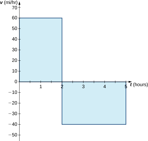
Suppose we want to know how far the car travels overall, regardless of direction. In this case, we want to know the area between the curve and the \(t\)-axis, regardless of whether that area is above or below the axis. This is called the total area.

Graphically, it is easiest to think of calculating total area by adding the areas above the axis and the areas below the axis (rather than subtracting the areas below the axis, as we did with net signed area). To accomplish this mathematically, we use the absolute value function. Thus, the total distance traveled by the car is

\[\int^2_0|60|\,dt+∫^5_2|−40|\,dt=∫^2_060\,dt+∫^5_240\,dt=120+120=240.\nonumber \]

Bringing these ideas together formally, we state the following definitions.

Example \(\PageIndex{3}\): Finding the Total Area

Find the total area between \(f(x)=x−2\) and the \(x\)-axis over the interval \([0,6].\)

Solution

Calculate the \(x\)-intercept as \((2,0)\) (set \(y=0,\) solve for \(x\)). To find the total area, take the area below the \(x\)-axis over the subinterval \([0,2]\) and add it to the area above the \(x\)-axis on the subinterval \([2,6]\) (Figure \(\PageIndex{7}\)).

We have

\[∫^6_0|(x−2)|\,dx=A_2+A_1. \nonumber \]

Then, using the formula for the area of a triangle, we obtain

\[A_2=\dfrac{1}{2}bh=\dfrac{1}{2}⋅2⋅2=2 \nonumber \]

\[A_1=\dfrac{1}{2}bh=\dfrac{1}{2}⋅4⋅4=8. \nonumber \]

The total area, then, is

\[A_1+A_2=8+2=10\,\text{units}^2. \nonumber \]

Properties of the Definite Integral

The properties of indefinite integrals apply to definite integrals as well. Definite integrals also have properties that relate to the limits of integration. These properties, along with the rules of integration that we examine later in this chapter, help us manipulate expressions to evaluate definite integrals.

Comparison Properties of Integrals

A picture can sometimes tell us more about a function than the results of computations. Comparing functions by their graphs as well as by their algebraic expressions can often give new insight into the process of integration. Intuitively, we might say that if a function \(f(x)\) is above another function \(g(x)\), then the area between \(f(x)\) and the \(x\)-axis is greater than the area between \(g(x)\) and the \(x\)-axis. This is true depending on the interval over which the comparison is made. The properties of definite integrals are valid whether \(a<b,\,a=b\), or \(a>b\). The following properties, however, concern only the case \(a≤b\), and are used when we want to compare the sizes of integrals.

Example \(\PageIndex{6}\): Comparing Two Functions over a Given Interval

Compare \(f(x)=\sqrt{1+x^2}\) and \(g(x)=\sqrt{1+x}\) over the interval \([0,1]\).

Solution

Graphing these functions is necessary to understand how they compare over the interval \([0,1].\) Initially, when graphed on a graphing calculator, \(f(x)\) appears to be above \(g(x)\) everywhere. However, on the interval \([0,1]\), the graphs appear to be on top of each other. We need to zoom in to see that, on the interval \([0,1],\,g(x)\) is above \(f(x)\). The two functions intersect at \(x=0\) and \(x=1\) (Figure \(\PageIndex{8}\)).

We can see from the graph that over the interval \([0,1],\,g(x)≥f(x)\). Comparing the integrals over the specified interval \([0,1],\) we also see that \(\displaystyle ∫^1_0g(x)\,dx≥∫^1_0f(x)\,dx\) (Figure \(\PageIndex{9}\)). The thin, red-shaded area shows just how much difference there is between these two integrals over the interval \([0,1].\)

Integrating Even and Odd Functions

We saw in Functions and Graphs that an even function is a function in which \(f(−x)=f(x)\) for all \(x\) in the domain—that is, the graph of the curve is unchanged when \(x\) is replaced with \(−x\). The graphs of even functions are symmetric about the \(y\)-axis. An odd function is one in which \(f(−x)=−f(x)\) for all \(x\) in the domain, and the graph of the function is symmetric about the origin.

Integrals of even functions, when the limits of integration are from \(−a\) to \(a\), involve two equal areas, because they are symmetric about the \(y\)-axis. Integrals of odd functions, when the limits of integration are similarly \([−a,a],\) evaluate to zero because the areas above and below the \(x\)-axis are equal.

Example \(\PageIndex{8}\): Integrating an Odd Function

Evaluate the definite integral of the odd function \(−5 \sin x\) over the interval \([−π,π].\)

Solution

The graph is shown in Figure \(\PageIndex{10}\). We can see the symmetry about the origin by the positive area above the \(x\)-axis over \([−π,0]\), and the negative area below the \(x\)-axis over \([0,π].\) we have

\[ \begin{align*} ∫^π_{−π}−5\sin x \,dx &=0. \end{align*}\]

Average Value of a Function

We often need to find the average of a set of numbers, such as an average test grade. Suppose you received the following test scores in your algebra class: 89, 90, 56, 78, 100, and 69. Your semester grade is your average of test scores and you want to know what grade to expect. We can find the average by adding all the scores and dividing by the number of scores. In this case, there are six test scores. Thus,

\[\dfrac{89+90+56+78+100+69}{6}=\dfrac{482}{6}≈80.33. \nonumber \]

Therefore, your average test grade is approximately 80.33, which translates to a B− at most schools.

Suppose, however, that we have a function \(v(t)\) that gives us the speed of an object at any time \(t\), and we want to find the object’s average speed. The function \(v(t)\) takes on an infinite number of values, so we can’t use the process just described. Fortunately, we can use a definite integral to find the average value of a function such as this.

Let \(f(x)\) be continuous over the interval \([a,b]\) and let \([a,b]\) be divided into n subintervals of width \(Δx=(b−a)/n\). Choose a representative \(x^∗_i\) in each subinterval and calculate \(f(x^∗_i)\) for \(i=1,2,…,n.\) In other words, consider each \(f(x^∗_i)\) as a sampling of the function over each subinterval. The average value of the function may then be approximated as

\[f_{ave} \approx \dfrac{f(x^∗_1)+f(x^∗_2)+⋯+f(x^∗_n)}{n}, \nonumber \]

which is basically the same expression used to calculate the average of discrete values.

But we know \(Δx=\dfrac{b−a}{n},\) so \(n=\dfrac{b−a}{Δx}\), and we get

\[f_{ave} \approx \dfrac{f(x^∗_1)+f(x^∗_2)+⋯+f(x^∗_n)}{n}=\dfrac{f(x^∗_1)+f(x^∗_2)+⋯+f(x^∗_n)}{\left(\dfrac{b−a}{Δx}\right)}. \nonumber \]

Following through with the algebra, the numerator is a sum that is represented as \(\sum_{i=1}^nf(x^∗_i),\) and we are dividing by a fraction. To divide by a fraction, invert the denominator and multiply. Thus, an approximate value for the average value of the function is given by

\[\dfrac{\sum_{i=1}^nf(x^∗_i)}{\left(\dfrac{b−a}{Δx}\right)}=\left(\dfrac{Δx}{b−a}\right)\sum_{i=1}^nf(x^∗_i)=\left(\dfrac{1}{b−a}\right)\sum_{i=1}^nf(x^∗_i)Δx. \nonumber \]

This is a Riemann sum. Then, to get the exact average value, take the limit as \(n\) goes to infinity. Thus, the average value of a function is given by

\[\dfrac{1}{b−a}\lim_{n→∞}\sum_{i=1}^nf(x_i)Δx=\dfrac{1}{b−a}∫^b_af(x)dx. \nonumber \]

Example \(\PageIndex{9}\): Finding the Average Value of a Linear Function

Find the average value of \(f(x)=x+1\) over the interval \([0,5].\)

Solution

First, graph the function on the stated interval, as shown in Figure \(\PageIndex{11}\).

The region is a trapezoid lying on its side, so we can use the area formula for a trapezoid \(A=\dfrac{1}{2}h(a+b),\) where \(h\) represents height, and \(a\) and \(b\) represent the two parallel sides. Then,

\(\displaystyle ∫^5_0x+1\,dx=\dfrac{1}{2}h(a+b)=\dfrac{1}{2}⋅5⋅(1+6)=\dfrac{35}{2}\).

Thus the average value of the function is

\(\displaystyle \dfrac{1}{5−0}∫^5_0x+1\,dx=\dfrac{1}{5}⋅\dfrac{35}{2}=\dfrac{7}{2}\).

Key Concepts

• The definite integral can be used to calculate net signed area, which is the area above the \(x\)-axis less the area below the \(x\)-axis. Net signed area can be positive, negative, or zero.
• The properties of definite integrals can be used to evaluate integrals.
• The area under the curve of many functions can be calculated using geometric formulas.
• The average value of a function can be calculated using definite integrals.

Key Equations

• Properties of the Definite Integral

\(\displaystyle∫^a_af(x)\,dx=0\)

\(\displaystyle∫^a_bf(x)\,dx=−∫^b_af(x)\,dx\)

\(\displaystyle∫^b_a[f(x)+g(x)]\,dx=∫^b_af(x)\,dx+∫^b_ag(x)\,dx\)

\(\displaystyle∫^b_a[f(x)−g(x)]\,dx=∫^b_af(x)\,dx−∫^b_ag(x)\,dx\)

\(\displaystyle∫^b_acf(x)\,dx=c∫^b_af(x)\,dx\), for constant \(c\)

\(\displaystyle∫^b_af(x)\,dx=∫^c_af(x)\,dx+∫^b_cf(x)\,dx\)

\(\displaystyle∫^a_{−a}f(x)\,dx=2∫^a_0f(x)\,dx\) for continuous even functions

\(\displaystyle∫^a_{−a}f(x)\,dx=0 \) for continuous odd functions

Glossary

average value of a function

(or \(f_{ave})\) the average value of a function on an interval can be found by calculating the definite integral of the function and dividing that value by the length of the interval

net signed area

the area between a function and the \(x\)-axis such that the area below the \(x\)-axis is subtracted from the area above the \(x\)-axis; the result is the same as the definite integral of the function

total area

total area between a function and the \(x\)-axis is calculated by adding the area above the \(x\)-axis and the area below the \(x\)-axis; the result is the same as the definite integral of the absolute value of the function