Opening the book…
In Section 0.2, we estimated the slope of a line tangent to the graph of a function at a point. At the end of Section 0.3, we constructed a new function that gave the slope of the line tangent to the graph of a given function at each point. In both cases, before we could calculate a slope, we had to estimate the tangent line from the graph of the given function, a method that required an accurate graph and good estimating. In this section we will begin to look at a more precise method of finding the slope of a tangent line that does not require a graph or any estimation by us. We will start with a non-applied problem and then look at two applications of the same idea.
The Slope of a Line Tangent to a Function at a Point
Our goal is to find a way of exactly determining the slope of the line that is tangent to a function (to the graph of the function) at a point in a way that does not require us to actually have the graph of the function
Let’s start with the problem of finding the slope of the line \(L\), which is tangent to \(f(x) = x^2\) at the point \((2,4)\):

We could estimate the slope of \(L\) from the graph above, but we won’t. Instead, we can see that the line through \((2,4)\) and \((3,9)\) on the graph of \(f\) is an approximation of the slope of the tangent line, and we can calculate that slope exactly:\[m = \frac{\Delta y}{\Delta x} = \frac{9-4}{3-2} = 5\]But \(m = 5\) is only an estimate of the slope of the tangent line — and not a very good estimate. It’s too big. We can get a better estimate by picking a second point on the graph of \(f\) closer to \((2,4)\) — the point \((2,4)\) is fixed and it must be one of the two points we use:

From the figure above we can see that the slope of the line through the points \((2,4)\) and \((2.5,6.25)\) is a better approximation of the slope of the tangent line at \((2,4)\):\[m = \frac{\Delta y}{\Delta x} = \frac{6.25 - 4}{2.5 - 2} = \frac{2.25}{0.5} = 4.5\]This is a better estimate, but still an approximation.
We can continue picking points closer and closer to \((2,4)\) on the graph of \(f\), and then calculating the slopes of the lines through each of these points \((x,y)\) and the point \((2,4)\):
| points to the left of \((2,4)\) | points to the right of \((2,4)\) | ||||
|---|---|---|---|---|---|
| \(x\) | \(y = x^2\) | slope | \(x\) | \(y = x^2\) | slope |
| \(1.5\) | \(2.25\) | \(3.5\) | \(3\) | \(9\) | \(5\) |
| \(1.9\) | \(3.61\) | \(3.9\) | \(2.5\) | \(6.25\) | \(4.5\) |
| \(1.99\) | \(3.9601\) | \(3.99\) | \(2.01\) | \(4.0401\) | \(4.01\) |
The only thing special about the \(x\)-values we picked is that they are numbers close — and very close — to \(x = 2\). Someone else might have picked other nearby values for \(x\). As the points we pick get closer and closer to the point \((2,4)\) on the graph of \(y = x^2\), the slopes of the lines through the points and \((2,4)\) are better approximations of the slope of the tangent line, and these slopes are getting closer and closer to \(4\).
What is the slope of the line through \((2,4)\) and \((x, y)\) for \(y = x^2\) and \(x = 1.994\)? For \(x = 2.0003\)?
- Answer
-
If \(x = 1.994\), then \(y = 3.976036\), so the slope between \((2, 4)\) and \((x ,y)\) is:\[\frac{4 - y}{2 - x} = \frac{4 - 3.976036}{2 - 1.994} = \frac{0.023964}{0.006} \approx 3.994\nonumber\]If \(x = 2.0003\), then \(y \approx 4.0012\), so the slope between \((2, 4)\) and \((x ,y)\) is:\[\frac{4 - y}{2 - x} = \frac{4 - 4.0012}{2 - 2.0003} = \frac{-0.0012}{-0.0003} \approx 4.0003\nonumber\]
We can bypass much of the calculating by not picking the points one at a time: let's look at a general point near \((2,4)\). Define \(x = 2 + h\) so \(h\) is the increment from \(2\) to \(x\):

If \(h\) is small, then \(x = 2 + h\) is close to \(2\) and the point \(\left(2+h, f(2+h) \right) = \left(2+h, (2+h)^2 \right)\) is close to \((2,4)\). The slope \(m\) of the line through the points \((2,4)\) and \(\left(2+h, (2+h)^2\right)\) is a good approximation of the slope of the tangent line at the point \((2,4)\): \begin{align*} m &= \frac{\Delta y}{\Delta x} = \frac{(2+h)^2 - 4}{(2+h) - 2} = \frac{(4 + 4h + h^2) - 4}{h}\\ &= \frac{4h + h^2}{h} = \frac{h(4 + h)}{h} = 4 + h \end{align*} If \(h\) is very small, then \(m = 4 + h\) is a very good approximation to the slope of the tangent line, and \(m = 4 + h\) also happens to be very close to the value \(4\). The value \(m = 4 + h\) is called the slope of the secant line through the two points \((2,4)\) and \(\left( 2+h, (2+h)^2 \right)\). The limiting value \(4\) of \(m = 4 + h\) as \(h\) gets smaller and smaller is called the slope of the tangent line to the graph of \(f\) at \((2,4)\).
Find the slope of the line tangent to \(f(x) = x^2\) at the point \((1,1)\) by evaluating the slope of the secant line through \((1,1)\) and \(\left( 1+h, f(1+h) \right)\) and then determining what happens as \(h\) gets very small.

Solution
The slope of the secant line through the points \((1,1)\) and \(\left( 1+h,f(1+h) \right)\) is: \begin{align*} m &= \frac{f(1+h) - 1}{( 1+h ) - 1} = \frac{( 1+h )^2 - 1}{h} = \frac{ (1 + 2h + h^2 ) - 1}{h}\\ &= \frac{2h + h^2}{h} = \frac{h(2+h)}{h} = 2 + h \end{align*} As \(h\) gets very small, the value of \(m\) approaches the value \(2\), the slope of tangent line at the point \((1,1)\).
Find the slope of the line tangent to the graph of \(y = f(x) = x^2\) at the point \((-1,1)\) by finding the slope of the secant line, \(m_{\mbox{sec}}\), through the points \((-1,1)\) and \(\left( -1+h, f( -1+h ) \right)\) and then determining what happens to \(m_{\mbox{sec}}\) as \(h\) gets very small.
- Answer
-
Computing \(m_{\mbox{sec}}\):\[\frac{f(-1 + h) - (1)}{(-1 + h) - (-1)} = \frac{(-1 + h)^2 - 1}{h} = \frac{1 - 2h + h^2 - 1}{h} = \frac{h(-2 + h)}{h} = -2 + h\nonumber\]As \(h \rightarrow 0\), \(m_{\mbox{sec}} = -2 + h \rightarrow -2\).
Falling Tomato
Suppose we drop a tomato from the top of a 100-foot building:

and record its position at various times during its fall:
| time (sec) | height (ft) |
|---|---|
| 0.0 | 100 |
| 0.5 | 96 |
| 1.0 | 84 |
| 1.5 | 64 |
| 2.0 | 36 |
| 2.5 | 0 |
Some questions about this situation are easy to answer directly from the table:
- How long did it take for the tomato to drop \(100\) feet? (\(2.5\) seconds)
- How far did the tomato fall during the first second? (\)100 - 84 = 16\) feet)
- How far did the tomato fall during the last second? (\\)64 - 0 = 64\) feet)
- How far did the tomato fall between \(t =0.5\) and \(t = 1\)? (\(\)96 - 84 = 12\) feet)
Other questions require a little calculation:
- What was the average velocity of the tomato during its fall?\[\mbox{average velocity} = \frac{\mbox{distance fallen}}{\mbox{total time}} = \frac{\Delta\mbox{position}}{\Delta\mbox{time}} = \frac{-100\mbox{ ft}}{2.5\mbox{ s}} = -40\, \frac{\mbox{ft}}{\mbox{sec}}\]
- What was the average velocity between \(t=1\) and \(t=2\) seconds?\[\mbox{average velocity} = \frac{\Delta\mbox{position}}{\Delta\mbox{time}} = \frac{36\mbox{ ft}- 84\mbox{ ft}}{2\mbox{ s} - 1\mbox{ s}} = \frac{-48\mbox{ ft}}{1\mbox{ s}} = -48\, \frac{\mbox{ft}}{\mbox{sec}}\]
Some questions are more difficult.
- How fast was the tomato falling \(1\) second after it was dropped?
This question is significantly different from the previous two questions about average velocity. Here we want the {\bf instantaneous velocity}, the velocity at an instant in time. Unfortunately, the tomato is not equipped with a speedometer, so we will have to give an approximate answer.
One crude approximation of the instantaneous velocity after \(1\) second is simply the average velocity during the entire fall, \(-40 \frac{\mbox{ft}}{\mbox{sec}}\). But the tomato fell slowly at the beginning and rapidly near the end, so this estimate may or may not be a good answer.
We can get a better approximation of the instantaneous velocity at \(t=1\) by calculating the average velocities over a short time interval near \(t = 1\). The average velocity between \(t = 0.5\) and \(t = 1\) is:\[\frac{-12\mbox{ feet}}{0.5 \mbox{ sec}} = -24\, \frac{\mbox{ft}}{\mbox{sec}}\]and the average velocity between \(t = 1\) and \(t = 1.5\) is\[\frac{-20\mbox{ feet}}{0.5 \mbox{ sec}} = -40\, \frac{\mbox{ft}}{\mbox{sec}}\]so we can be reasonably sure that the instantaneous velocity is between \(-24\, \frac{\mbox{ft}}{\mbox{sec}}\) and \(-40\, \frac{\mbox{ft}}{\mbox{sec}}\).
In general, the shorter the time interval over which we calculate the average velocity, the better the average velocity will approximate the instantaneous velocity. The average velocity over a time interval is:\[\frac{\Delta \mbox{position}}{\Delta \mbox{time}}\]which is the slope of the secant line through two points on the graph of height versus time:

\begin{align*}\mbox{average velocity } &= \frac{\Delta \mbox{position}}{\Delta \mbox{time}}\\ &= \mbox{slope of the secant line through two points}\end{align*}
The instantaneous velocity at a particular time and height is the slope of the tangent line to the graph at the point given by that time and height.
instantaneous velocity = slope of the line tangent to the graph
Estimate the instantaneous velocity of the tomato \(2\) seconds after it was dropped.
- Answer
-
The average velocity between \(t = 1.5\) and \(t = 2.0\) is: \[\frac{36 - 64 \mbox{ feet}}{2.0 - 1.5 \mbox{ sec}} = -56\, \frac{\mbox{feet}}{\mbox{sec}}\nonumber\]The average velocity between \(t = 2.0\) and \(t = 2.5\) is: \[\frac{0 - 36 \mbox{ feet}}{2.5 - 2.0 \mbox{ sec}} = -72\, \frac{\mbox{feet}}{\mbox{sec}}\nonumber\]The velocity at \(t = 2.0\) is somewhere between \(-56\, \frac{\mbox{feet}}{\mbox{sec}}\) and \(-72\, \frac{\mbox{feet}}{\mbox{sec}}\), probably around the middle of this interval:\[\frac{(-56) + (-72)}{2} = -64\, \frac{\mbox{feet}}{\mbox{sec}}\nonumber\]
Growing Bacteria
Suppose we set up a machine to count the number of bacteria growing on a Petri plate:

At first there are few bacteria, so the population grows slowly. Then there are more bacteria to divide, so the population grows more quickly. Later, there are more bacteria and less room and nutrients available for the expanding population, so the population grows slowly again. Finally, the bacteria have used up most of the nutrients and the population declines as bacteria die.
The population graph can be used to answer a number of questions:
- What is the bacteria population at time \(t = 3\) days? (about \(500\) bacteria)
- What is the population increment from \(t = 3\) to \(t = 10\) days? (about \(4,000\) bacteria)
- What is the {\bf rate} of population growth from \(t = 3\) to \(t = 10\) days?
To answer this last question, we compute the average change in population during that time: \begin{align*} \mbox{average change }&\mbox{in population} = \frac{\mbox{change in population}}{\mbox{change in time}}\\ &= \frac{\Delta\mbox{population}}{\Delta\mbox{time}} = \frac{4000\mbox{ bacteria}}{7\mbox{ days}} \approx 570\, \frac{\mbox{bacteria}}{\mbox{day}} \end{align*} This is the slope of the secant line through \((3, 500)\) and \((10, 4500)\).
average population growth rate = \(\displaystyle \frac{\Delta \mbox{population}}{\Delta \mbox{time}}\) \(=\) slope of the secant line through two points
Now for a more difficult question:
- What is the rate of population growth on the third day, at \(t = 3\)?
This question asks for the instantaneous rate of population change, the slope of the line tangent to the population curve at \((3, 500)\). If we sketch a line approximately tangent to the curve at \((3, 500)\) and pick two points near the ends of the tangent line segment:

we can estimate that the instantaneous rate of population growth is approximately \(320~\frac{\mbox{bacteria}}{\mbox{day}}\).
instantaneous population growth rate \(=\) slope of the line tangent to the graph
Find approximate values for:
- the average change in population between \(t = 9\) and \(t = 13\).
- the rate of population growth at \(t = 9\) days.
- Answer
-
- When \(t = 9\) days, the population is approximately \(P = 4,200\) bacteria. When \(t = 13\), \(P \approx 5,000\). The average change in population is approximately:\[\frac{5000 - 4200 \mbox{ bacteria}}{13 - 9 \mbox{ days}} = \frac{800 \mbox{ bacteria}}{4 \mbox{ days}} = 200\, \frac{\mbox{bacteria}}{\mbox{day}}\nonumber\]
- To find the rate of population growth at \(t = 9\) days, sketch the line tangent to the population curve at the point \((9, 4200)\) and then use \((9, 4200)\) and another point on the tangent line to calculate the slope of the line. Using the approximate values \((5, 2800)\) and \((9, 4200)\), the slope of the tangent line at the point \((9, 4200)\) is approximately:\[\frac{4200 - 2800 \mbox{ bacteria}}{9 - 5 \mbox{ days}} = \frac{1400 \mbox{ bacteria}}{4 \mbox{ days}} \approx 350\, \frac{\mbox{bacteria}}{\mbox{day}}\nonumber\]
The tangent line problem, the instantaneous velocity problem and the instantaneous growth rate problem are all similar. In each problem we wanted to know how rapidly something was changing at an instant in time, and each problem turned out to involve finding the slope of a tangent line. The approach in each problem was also the same: find an approximate solution and then examine what happens to the approximate solution over shorter and shorter intervals. We will often use this approach of finding a limiting value, but before we can use it effectively we need to describe the concept of a limit with more precision.
Problems
-
- What is the slope of the line through \((3,9)\) and \((x, y)\) for \(y = x^2\) when:
- \(x = 2.97\)?
- \(x = 3.001\)?
- \(x = 3+h\)?
- What happens to this last slope when \(h\) is very small (close to \(0\))?
- Sketch the graph of \(y = x^2\) for \(x\) near \(3\).
- What is the slope of the line through \((3,9)\) and \((x, y)\) for \(y = x^2\) when:
-
- What is the slope of the line through \((-2,4)\) and \((x, y)\) for \(y = x^2\) when:
- \(x = -1.98\)?
- \(x = -2.03\)?
- \(x = -2+h\)?
- What happens to this last slope when \(h\) is very small (close to \(0\))?
- Sketch the graph of \(y = x^2\) for \(x\) near \(-2\).
- What is the slope of the line through \((-2,4)\) and \((x, y)\) for \(y = x^2\) when:
-
- What is the slope of the line through \((2,4)\) and \((x, y)\) for \(y = x^2 + x - 2\) when:
- \(x = 1.99\)?
- \(x = 2.004\)?
- \(x = 2+h\)?
- What happens to this last slope when \(h\) is very small (close to \(0\))?
- Sketch the graph of \(y = x^2 + x - 2\) for \(x\) near \(2\).
- What is the slope of the line through \((2,4)\) and \((x, y)\) for \(y = x^2 + x - 2\) when:
-
- What is the slope of the line through \((-1,-2)\) and \((x, y)\) for \(y = x^2 + x - 2\) when:
- \(x = -0.98\)?
- \(x = -1.03\)?
- \(x = -1+h\)?
- What happens to this last slope when \(h\) is very small (close to \(0\))?
- Sketch the graph of \(y = x^2 + x - 2\) for \(x\) near \(-1\).
- What is the slope of the line through \((-1,-2)\) and \((x, y)\) for \(y = x^2 + x - 2\) when:
- The figure below shows the temperature during a day in Ames:
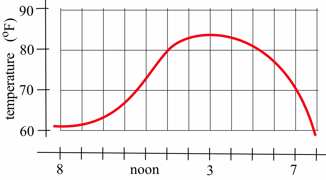
- What was the average change in temperature from 9 a.m.\ to 1 p.m.?
- Estimate how fast the temperature was rising at 10 a.m.\ and at 7 p.m.
- The figure below shows the distance of a car from a measuring position located on the edge of a straight road:

- What was the average velocity of the car from \(t = 0\) to \(t = 30\) seconds?
- What was the average velocity from \(t = 10\) to \(t = 30\) seconds?
- About how fast was the car traveling at \(t = 10\) seconds? At \(t = 20\)? At \(t = 30\)?
- What does the horizontal part of the graph between \(t = 15\) and \(t = 20\) seconds tell you?
- What does the negative velocity at \(t = 25\) represent?
- The figure below shows the distance of a car from a measuring position located on the edge of a straight road::

- What was the average velocity of the car from \(t = 0\) to \(t = 20\) seconds?
- What was the average velocity from \(t = 10\) to \(t = 30\) seconds?
- About how fast was the car traveling at \(t = 10\) seconds? At \(t = 20\)? At \(t = 30\)?
- The figure below shows the composite developmental skill level of chessmasters at different ages as determined by their performance against other chessmasters.

(From ``Rating Systems for Human Abilities,'' by W.H. Batchelder and R.S. Simpson, 1988. UMAP Module 698.)- At what age is the “typical” chessmaster playing the best chess?
- At approximately what age is the chessmaster’s skill level increasing most rapidly?
- Describe the development of the ``typical'' chessmaster's skill in words.
- Sketch graphs that you {\bf think} would reasonably describe the performance levels versus age for an athlete, a classical pianist, a rock singer, a mathematician and a professional in your major field.
- Define \(A(x)\) to be the area bounded by the \(t\)- (horizontal) and \(y\)-axes, the horizontal line \(y = 3\), and the vertical line at \(x\):

For example, \(A(4) = 12\) is the area of the \(4 \times 3\) rectangle.- Evaluate \(A(0)\), \(A(1)\), \(A(2)\), \(A(2.5)\) and \(A(3)\).
- What area would \(A(4) - A(1)\) represent?
- Graph \(y = A(x)\) for \(0 \leq x \leq 4\).
- Define \(A(x)\) to be the area bounded by the \(t\)- (horizontal) and \(y\)-axes, the line \(y = t + 1\), and the vertical line at \(x\):

For example, \(A(4) = 12\).- Evaluate \(A(0)\), \(A(1)\), \(A(2)\), \(A(2.5)\) and \(A(3)\).
- What area would \(A(3) - A(1)\) represent in the figure?
- Graph \(y = A(x)\) for \(0 \leq x \leq 4\).
This page titled 1.0: Tangent Lines, Velocities and Graphs was last modified on Wed, 28 Jan 2026 21:01:13 GMT and is shared under a CC BY-NC-SA 4.0 license and was authored, remixed, and/or curated by Dale Hoffman, edited and updated by Jeff Eldridge.
The book could not be loaded just now.