Opening the book…
A line integral gives us the ability to integrate multivariable functions and vector fields over arbitrary curves in a plane or in space. There are two types of line integrals: scalar line integrals and vector line integrals. Scalar line integrals are integrals of a scalar function over a curve in a plane or in space. Vector line integrals are integrals of a vector field over a curve in a plane or in space. Let’s look at scalar line integrals first.
A scalar line integral is defined just as a single-variable integral is defined, except that for a scalar line integral, the integrand is a function of more than one variable and the domain of integration is a curve in a plane or in space, as opposed to a curve on the \(x\)-axis.
For a scalar line integral, we let \(C\) be a smooth curve in a plane or in space and let \(f\) be a function with a domain that includes \(C\). We chop the curve into small pieces. For each piece, we choose point \(P\) in that piece and evaluate \(f\) at \(P\). (We can do this because all the points in the curve are in the domain of \(f\).) We multiply \(f(P)\) by the arc length of the piece \(\Delta s\), add the product \(f(P)\Delta s\) over all the pieces, and then let the arc length of the pieces shrink to zero by taking a limit. The result is the scalar line integral of the function over the curve.
For a formal description of a scalar line integral, let \(C\) be a smooth curve in space given by the parameterization \(\vecs r(t)=⟨x(t),y(t),z(t)⟩\), \(a≤t≤b\). Let \(f(x,y,z)\) be a function with a domain that includes curve \(C\). To define the line integral of the function \(f\) over \(C\), we begin as most definitions of an integral begin: we chop the curve into small pieces. Partition the parameter interval \([a,b]\) into \(n\) subintervals \([t_{i−1},t_i]\) of equal width for \(1≤i≤n\), where \(t_0=a\) and \(t_n=b\) (Figure \(\PageIndex{1}\)). Let \(t_{i}^*\) be a value in the \(i^{th}\) interval \([t_{i−1},t_i]\). Denote the endpoints of \(\vecs r(t_0)\), \(\vecs r(t_1)\),…, \(\vecs r(t_n)\) by \(P_0\),…, \(P_n\). Points Pi divide curve \(C\) into \(n\) pieces \(C_1\), \(C_2\),…, \(C_n\), with lengths \(\Delta s_1\), \(\Delta s_2\),…, \(\Delta s_n\), respectively. Let \(P_{i}^*\) denote the endpoint of \(\vecs r(t_{i}^*)\) for \(1≤i≤n\). Now, we evaluate the function \(f\) at point \(P_{i}^*\) for \(1≤i≤n\). Note that \(P_{i}^*\) is in piece \(C_i\), and therefore \(P_{i}^*\) is in the domain of \(f\). Multiply \(f(P_{i}^*)\) by the length \(\Delta s_i\) of \(C_i\), which gives the area of the “sheet” with base \(C_i\), and height \(f(P_{i}^{*})\). This is analogous to using rectangles to approximate area in a single-variable integral. Now, we form the sum \(\displaystyle \sum_{i=1}^{n} f(P_{i}^{*})\,\Delta s_i\).
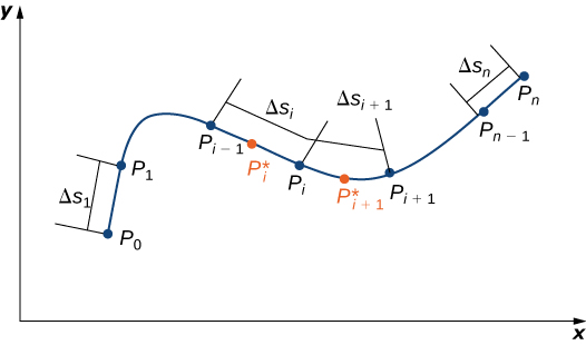
Note the similarity of this sum versus a Riemann sum; in fact, this definition is a generalization of a Riemann sum to arbitrary curves in space. Just as with Riemann sums and integrals of form \(\displaystyle \int_{a}^{b}g(x)\,dx\), we define an integral by letting the width of the pieces of the curve shrink to zero by taking a limit. The result is the scalar line integral of \(f\) along \(C\).
You may have noticed a difference between this definition of a scalar line integral and a single-variable integral. In this definition, the arc lengths \(\Delta s_1\), \(\Delta s_2\),…, \(\Delta s_n\) aren’t necessarily the same; in the definition of a single-variable integral, the curve on the \(x\)-axis is partitioned into pieces of equal length. This difference does not have any effect in the limit. As we shrink the arc lengths to zero, their values become close enough that any small difference becomes irrelevant.
Let \(f\) be a function with a domain that includes the smooth curve \(C\) that is parameterized by \(\vecs r(t)=⟨x(t),y(t),z(t)⟩\), \(a≤t≤b\). The scalar line integral of \(f\) along \(C\) is
\[\int_C f(x,y,z) \,ds=\lim_{n\to\infty}\sum_{i=1}^{n}f(P_{i}^{*})\,\Delta s_i \nonumber \]
if this limit exists (\(t_i ^{*}\) and \(\Delta s_i\) are defined as in the previous paragraphs). If \(C\) is a planar curve, then \(C\) can be represented by the parametric equations \(x=x(t)\), \(y=y(t)\), and \(a≤t≤b\). If \(C\) is smooth and \(f(x,y)\) is a function of two variables, then the scalar line integral of \(f\) along \(C\) is defined similarly as
\[\int_C f(x,y) \,ds=\lim_{n\to\infty}\sum_{i=1}^{n} f(P_{i}^{*})\,\Delta s_i \nonumber \]
if this limit exists.
If \(f\) is a continuous function on a smooth curve \(C\), then \(\displaystyle \int_C f \,ds\) always exists. Since \(\displaystyle \int_C f \,ds\) is defined as a limit of Riemann sums, the continuity of \(f\) is enough to guarantee the existence of the limit, just as the integral \(\displaystyle \int_{a}^{b}g(x)\,dx\) exists if \(g\) is continuous over \([a,b]\).
Before looking at how to compute a line integral, we need to examine the geometry captured by these integrals. Suppose that \(f(x,y)≥0\) for all points \((x,y)\) on a smooth planar curve \(C\). Imagine taking curve \(C\) and projecting it “up” to the surface defined by \(f(x,y)\), thereby creating a new curve \(C′\) that lies in the graph of \(f(x,y)\). Now we drop a “sheet” from \(C′\) down to the \(xy\)-plane. The area of this sheet is \(\displaystyle \int_C f(x,y)ds\). If \(f(x,y)≤0\) for some points in \(C\), then the value of \(\displaystyle \int_C f(x,y)\,ds\) is the area above the \(xy\)-plane less the area below the \(xy\)-plane. (Note the similarity with integrals of the form \(\displaystyle \int_{a}^{b}g(x)\,dx\).)
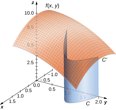
From this geometry, we can see that line integral \(\displaystyle \int_C f(x,y)\,ds\) does not depend on the parameterization \(\vecs r(t)\) of \(C\). As long as the curve is traversed exactly once by the parameterization, the area of the sheet formed by the function and the curve is the same. This same kind of geometric argument can be extended to show that the line integral of a three-variable function over a curve in space does not depend on the parameterization of the curve.
Consider \(\displaystyle \int_C 2\,ds\), where \(C\) is the upper half of the unit circle.
The integrand is \(f(x,y)=2\). The graph of \(f(x,y)=2\), curve C, and the sheet formed by them are provided below. Notice that this sheet has the same area as a rectangle with width \(\pi\) and length \(2\). Therefore, \(\displaystyle \int_C 2 \,ds=2\pi\,\text{units}^2\)
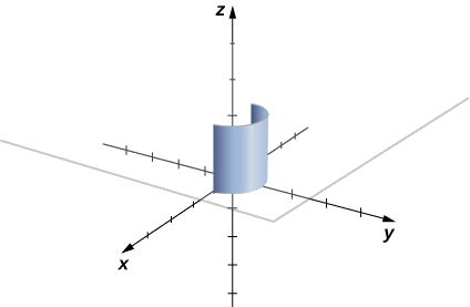
To see that \(\displaystyle \int_C 2 \,ds=2\pi\) using the definition of line integral, we let \(\vecs r(t)\) be a parameterization of \(C\). Then, \(f(\vecs r(t_i))=2\) for any number \(t_i\) in the domain of \(\vecs r\). Therefore,
\[ \int_C f \,ds =\lim_{n\to\infty}\sum_{i=1}^{n} f(\vecs r(t_{i}^{*}))\,\Delta s_i =\lim_{n\to\infty}\sum_{i=1}^{n}2\,\Delta s_i =2\lim_{n\to\infty}\sum_{i=1}^{n}\,\Delta s_i =2(\text{length}\space \text{of}\space C) =2\pi \,\text{units}^2 \nonumber \]
Note that in a scalar line integral, the integration is done with respect to arc length \(s\), which can make a scalar line integral difficult to calculate. To make the calculations easier, we can translate \(\displaystyle \int_C f\,ds\) to an integral with a variable of integration that is \(t\).
Let \(\vecs r(t)=⟨x(t),y(t),z(t)⟩\) for \(a≤t≤b\) be a parameterization of \(C\). Since we are assuming that \(C\) is smooth, \(\vecs r′(t)=⟨x′(t),y′(t),z′(t)⟩\) is continuous for all \(t\) in \([a,b]\). In particular, \(x′(t)\), \(y′(t)\), and \(z′(t)\) exist for all \(t\) in \([a,b]\). According to the arc length formula, we have
\[\text{length}(C_i)=\Delta s_i=\int_{t_{i−1}}^{t_i} ‖\vecs r′(t)‖\,dt \nonumber \]
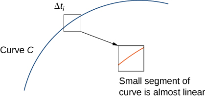
If width \(\Delta t_i=t_i−t_{i−1}\) is small, then function \(\displaystyle \int_{t_{i−1}}^{t_i} ‖\vecs r′(t)‖\,dt\,≈\,‖\vecs r′(t_i^*)‖\,\Delta t_i\), \(‖\vecs r′(t)‖\) is almost constant over the interval \([t_{i−1},t_i]\). Therefore,
\[\int_{t_{i−1}}^{t_i} ‖\vecs r′(t)‖\,dt\,≈\,‖\vecs r′(t_{i}^{*})‖\,\Delta t_i, \text{ and therefore } \sum_{i=1}^{n} f(\vecs r(t_i^*))\,\Delta s_i\approx\sum_{i=1}^{n} f(\vecs r(t_{i}^{*})) ‖\vecs r′(t_{i}^{*})‖\,\Delta t_i \nonumber \]
Note that
\[\lim_{n\to\infty}\sum_{i=1}^{n} f(\vecs r(t_i^*))‖\vecs r′(t_{i}^{*})‖\,\Delta t_i=\int_a^b f(\vecs r(t))‖\vecs r′(t)‖\,dt \nonumber \]
In other words, as the widths of intervals \([t_{i−1},t_i]\) shrink to zero, the sum \(\displaystyle \sum_{i=1}^{n} f(\vecs r(t_i^{*}))‖\vecs r′(t_{i}^{*})‖\,\Delta t_i\) converges to the integral \(\displaystyle \int_{a}^{b}f(\vecs r(t))‖\vecs r′(t)‖\,dt\).
Let \(f\) be a continuous function with a domain that includes the smooth curve \(C\) with parameterization \(\vecs r(t)\), for \(a≤t≤b\). Then
\[\int_C f \,ds=\int_{a}^{b} f(\vecs r(t))‖\vecs r′(t)‖\,dt\nonumber \]
Since \( ‖\vecs r′(t)‖=\sqrt{{(x′(t))}^2+{(y′(t))}^2+{(z′(t))}^2} \) we obtain the following theorem, which we use to compute scalar line integrals.
Let \(f\) be a continuous function with a domain that includes the smooth curve \(C\) with parameterization \(\vecs r(t)=⟨x(t),y(t),z(t)⟩\), \(a≤t≤b\). Then
\[\int_C f(x,y,z) \,ds=\int_{a}^{b} f(\vecs r(t))\sqrt{({x′(t))}^2+{(y′(t))}^2+{(z′(t))}^2} \,dt \nonumber \]
Similarly,
\[\int_C f(x,y) \,ds=\int_{a}^{b}f(\vecs r(t))\sqrt{{(x′(t))}^2+{(y′(t))}^2} \,dt \nonumber \]
if \(C\) is a planar curve and \(f\) is a function of two variables.
Note that a consequence of this theorem is the equation \(ds=‖\vecs r′(t)‖ \,dt\). In other words, the change in arc length can be viewed as a change in the \(t\)-domain, scaled by the magnitude of vector \(\vecs r′(t)\).
Find the value of integral \(\displaystyle \int_C(x^2+y^2+z) \,ds\), where \(C\) is part of the helix parameterized by
(a) \(\vecs r(t)=⟨\cos (t),\sin (t),t⟩\) for \(0≤t≤2\pi\)
(b) \(\vecs r(t)=⟨\cos(2t),\sin(2t),2t⟩\) for \(0≤t≤π\)
Solution
(a) To compute a scalar line integral, we start by converting the variable of integration from arc length \(ds\) to \(dt\). Note that
\[f(x,y,z)=x^2+y^2+z \implies f(\cos(t),\sin(t),t)={\cos}^2 (t)+{\sin}^2 (t)+t=1+t \nonumber \]
and
\[\sqrt{{(x′(t))}^2+{(y′(t))}^2+{(z′(t))}^2} =\sqrt{{(−\sin(t))}^2+{\cos}^2(t)+1} =\sqrt{2} \nonumber \]
Therefore,
\[ \int_C(x^2+y^2+z) \,ds=\int_{0}^{2\pi} (1+t)\sqrt{2} \,dt =\left[t\sqrt{2}+\dfrac{t^2\sqrt{2}}{2}\right]\Bigg|_{0}^{2\pi}=\boxed{2\pi \sqrt{2} +2\pi^2 \sqrt{2}} \nonumber \]
(b) We repeat with our new parameterization:
\[f(x,y,z)=x^2+y^2+z \implies f(\cos(2t),\sin(2t),2t)={\cos}^2 (2t)+{\sin}^2 (2t)+2t=1+2t \nonumber \]
and
\[\sqrt{{(x′(t))}^2+{(y′(t))}^2+{(z′(t))}^2} =\sqrt{ (-2\sin(2t))^2+(2\cos(2t))^2+(2)^2} =\sqrt{8} \nonumber \]
Therefore,
\[ \int_C(x^2+y^2+z) \,ds=\int_{0}^{\pi} (1+2t)\sqrt{8} \,dt =\left[t\sqrt{8}+ t^2\sqrt{8} \right]\Big|_{0}^{\pi}=\pi \sqrt{8} +\pi^2 \sqrt{8}=\boxed{ 2\pi \sqrt{2} +2\pi^2 \sqrt{2}} \nonumber \]
Notice that these solutions agree. Changing the parameterization did not change the value of the line integral. Scalar line integrals are independent of parameterization, as long as the curve is traversed exactly once by the parameterization.
Now that we can evaluate line integrals, we can use them to calculate arc length. If \(f(x,y,z)=1\), then
\[\begin{align*} \int_C f(x,y,z) \,ds &=\lim_{n\to\infty} \sum_{i=1}^{n} f(t_{i}^{*}) \,\Delta s_i \\[4pt] &=\lim_{n\to\infty} \sum_{i=1}^{n} \,\Delta s_i \\[4pt] &=\lim_{n\to\infty} \text{length} (C)\\[4pt] &=\text{length} (C) \end{align*}\]
Therefore, \(\displaystyle \int_C 1 \,ds\) is the arc length of \(C\).
Find the length of the wire that can be modeled with the parameterization \(\vecs r(t)=\left\langle \cos (t),\sin (t),\frac{2}{3} t^{\frac{3}{2}}\right\rangle \), for \(0≤t≤4\pi\)
Solution
The length of the wire is given by \(\displaystyle \int_C 1 \,ds\), where \(C\) is the curve with parameterization \(\vecs r\). Therefore,
\[\text{Length} =\int_C 1 \,ds=\int_{0}^{4\pi} ||\vecs r′(t)||\,dt=\int_{0}^{4\pi} \sqrt{\left(−\sin (t)\right)^2+\left(\cos(t)\right)^2+t}\,dt =\int_{0}^{4\pi} \sqrt{1+t}\, dt =\dfrac{2{(1+t)}^{\frac{3}{2}}}{3} \Bigg|_{0}^{4\pi} =\boxed{\frac{2}{3}\left((1+4\pi)^{\frac{3}{2}}−1\right)} \nonumber \]
A second type of line integrals is vector line integrals, in which we integrate along a curve through a vector field. For example, let
\[\vecs F(x,y,z)=P(x,y,z)\,\hat{\mathbf i}+Q(x,y,z)\,\hat{\mathbf j}+R(x,y,z)\,\hat{\mathbf k} \nonumber \]
be a continuous vector field in \(ℝ^3\) that represents a force on a particle, and let \(C\) be a smooth curve in \(ℝ^3\) contained in the domain of \(\vecs F\). How would we compute the work done by \(\vecs F\) in moving a particle along \(C\)?
To answer this question, first note that a particle could travel in two directions along a curve: a forward direction and a backward direction. The work done by the vector field depends on the direction in which the particle is moving. Therefore, we must specify a direction along curve \(C\); such a specified direction is called an orientation of a curve. The specified direction is called the "positive" direction along \(C\); the opposite direction is the "negative" direction along \(C\). When \(C\) has been given an orientation, \(C\) is called an oriented curve. The work done on the particle depends on the direction along the curve in which the particle is moving.
A closed curve is one for which there exists a parameterization \(\vecs r(t)\), \(a≤t≤b\), such that \(\vecs r(a)=\vecs r(b)\), and the curve is traversed exactly once. In other words, the parameterization is one-to-one on the domain \((a,b)\).
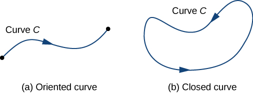
(b) A closed oriented curve.
Let \(\vecs r(t)\) be a parameterization of \(C\) for \(a≤t≤b\) such that the curve is traversed exactly once by the particle and the particle moves in the positive direction along \(C\). Divide the parameter interval \([a,b]\) into n subintervals \([t_{i−1},t_i]\), \(0≤i≤n\), of equal width. Denote the endpoints of \(r(t_0)\), \(r(t_1)\),…, \(r(t_n)\) by \(P_0\),…,\(P_n\). Points \(P_i\) divide \(C\) into n pieces. Denote the length of the piece from \(P_{i−1}\) to \(P_i\) by \(\Delta s_i\). For each \(i\), choose a value \(t_i^*\) in the subinterval \([t_{i−1},t_i]\). Then, the endpoint of \(\vecs r(t_i^*)\) is a point in the piece of \(C\) between \(P_{i−1}\) and \(P_i\). If \(\Delta s_i\) is small, then as the particle moves from \(P_{i−1}\) to \(P_i\) along \(C\), it moves approximately in the direction of \(\vecs{T}(P_i^*)=\dfrac{ \vecs{r}'(P_i^*) }{ \| \vecs{r}'(P_i^*)\| } \), the unit tangent vector at the endpoint of \(\vecs r(P_i^*)\).
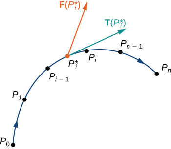
Then, the work done by the force vector field in moving the particle from \(P_{i−1}\) to \(P_i\) is \(\left\| \text{proj}_{\vecs{T}(P_i^*)}\left( \vecs{F}(P_i^*)\right)\right\|\Delta s_i=\vecs F(P_i^*)·( \vecs T(P_i^*))\Delta s_i\), so the total work done along \(C\) is
\[\sum_{i=1}^n \vecs F(P_i^*)·(\Delta s_i \vecs T(P_i^*))=\sum_{i=1}^n \vecs F(P_i^*)·\vecs T(P_i^*)\,\Delta s_i \nonumber \]
Let \(\vecs{F}\) be a vector field with a domain that includes the smooth curve \(C\) that is parameterized by \(\vecs r(t)\), \(a≤t≤b\). The line integral of \(\vecs{F}\) along \(C\) is
\[\int_C \vecs{F}(x,y,z) \cdot d\vecs{r}=\lim_{n\to\infty}\sum_{i=1}^n \vecs F(P_i^*)·\vecs T(P_i^*)\,\Delta s_i\nonumber \]
if this limit exists.
Letting the arc length of the pieces of \(C\) get arbitrarily small by taking a limit as \(n\rightarrow \infty\) gives us the work done by the field in moving the particle along \(C\). Therefore, the work done by \(\vecs{F}\) in moving the particle in the positive direction along \(C\) is defined as
\[W=\int_C \vecs{F} \cdot \dfrac{\vecs{r}' }{\|\vecs{r}'\|}\,ds=\int_a^b \vecs{F}(\vecs{r}(t))\cdot \vecs{r}'(t)\,dt \nonumber \]
which gives us the concept of a vector line integral.
The vector line integral of vector field \(\vecs{F}\) along oriented smooth curve \(C\) parameterized by \(\vecs{r}(t)\) on \(a\le t\le b\) is
\[\int_C \vecs{F} \cdot d\vecs{r}=\int_a^b \vecs{F}(\vecs{r}(t))\cdot \vecs{r}'(t)\,dt\nonumber \]
Let \(\vecs F=⟨−y,x⟩\) and find the value of integral \(\displaystyle \int_C \vecs{F} \cdot d\vecs{r}\), where \(C\) is
(a) the semicircle parameterized by \(\vecs{r}(t)=⟨\cos (t),\sin (t)⟩\), for \(0≤t≤\pi\)
(b) the semicircle parameterized by \(\vecs r(t)=⟨ -\cos(t),\sin (t)⟩\), for \(0≤t≤\pi\)
For the curve in (a), we are given \(\vecs{r}(t)=\langle \cos(t),\sin(t)\rangle \) so differentiating each component gives \(\vecs{r}'(t)=\langle -\sin(t), \cos(t)\rangle\)
Replacing \(x=\cos(t)\) and \(y=\sin(t)\) into \(\vecs{F}(x,y)\) we get \( \vecs{F}(\vecs{r}(t))=\left\langle -\sin(t), \cos(t)\right\rangle\)
Therefore,
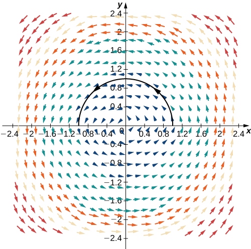
\[ \int_C \vecs{F} \cdot d\vecs{r} =\int_0^{\pi}⟨−\sin (t),\cos (t)⟩·⟨−\sin (t),\cos (t)⟩ \,dt =\int_0^{\pi} \sin^2(t)+\cos^2(t) \,dt =\int_0^{\pi}1 \,dt=\pi \nonumber \]
If we look at a sketch of this curve over the vector field \(\vecs{F}\), we can see that indeed these force arrows push in the same direction as the oriented curve \(C\). Thus, the "current" \(\vecs{F}\) "helps" a person swimming along this path by a positive amount:
In (b), we are given \(\vecs{r}(t) =\langle -\cos(t),\sin(t) \rangle \) so differentiating each component gives \(\vecs{r}'(t)=\langle \sin(t), \cos(t)\rangle\)
Replacing \(x=-\cos(t)\) and \(y=\sin(t)\) into \(\vecs{F}(x,y)\) we get \( \vecs{F}(\vecs{r}(t))=\left\langle -\sin(t), -\cos(t)\right\rangle\)
Therefore,
\[ \int_C \vecs{F} \cdot d\vecs{r} =\int_0^{\pi}⟨−\sin (t),-\cos (t)⟩·⟨\sin (t),\cos (t)⟩ \,dt =\int_0^{\pi} -\sin^2(t)-\cos^2(t) \,dt =\int_0^{\pi}-1 \,dt=-\pi \nonumber \]
Notice this is the same curve as part (a), just traversed in the opposite direction. In this case, the swimmer is fighting against the "current" of \(\vecs{F}\), so they are "helped" by a negative amount.
Let \(C\) be an oriented curve and let \(-C\) denote the same curve but with the orientation reversed. Then, the previous two examples illustrate the following fact:
\[\int_{-C} \vecs{F} \cdot d\vecs{r}=−\int_C\vecs{F} \cdot d\vecs{r} \nonumber \]
That is, reversing the orientation of a curve changes the sign of a line integral.
Another standard notation for integral \(\displaystyle \int_C \vecs{F} \cdot d\vecs{r}\) is \(\displaystyle \int_C P\,dx+Q\,dy+R \,dz\). In this notation, \(P,\, Q\), and \(R\) are functions, and we think of \(d\vecs{r}\) as vector \(⟨dx,dy,dz⟩\). To justify this convention, recall that \(d\vecs{r}=\vecs r′(t) \,dt=\left\langle\dfrac{dx}{dt},\dfrac{dy}{dt},\dfrac{dz}{dt}\right\rangle\,dt=\langle dx, dy, dz\rangle\). Therefore,
\[\int_C \vecs{F} \cdot d\vecs{r}=\int_C ⟨P,Q,R⟩·⟨dx,dy,dz⟩=\int_C P\,dx+Q\,dy+R\,dz =\int_a^b\left(P\big(\vecs r(t)\big)\dfrac{dx}{dt}+Q\big(\vecs r(t)\big)\dfrac{dy}{dt}+R\big(\vecs r(t)\big)\dfrac{dz}{dt}\right)\,dt \nonumber \]
Find the value of integral \(\displaystyle \int_C (3z\,dx-5x\,dy+3y\,dz)\), where \(C\) is the curve parameterized by \(\vecs r(t)=⟨t^2,\sqrt{t},t⟩\), for \(1≤t≤4\).
Solution
Since \(\vecs{r}(t)=\langle t^2,\sqrt{t},t\rangle\), we have \(\vecs{r}'(t)=\left\langle 2t,\dfrac{1}{2\sqrt{t}},1\right\rangle \)
We use the equation derived above to get:
\[\begin{align*} \int_C 3z\,dx-5x\,dy+3y\,dz &=\int_1^4 \left(3t\cdot 2t-5t^2\cdot \frac{1}{2\sqrt{t}}+3\sqrt{t}\cdot 1\right)\,dt \\[4pt] &=\int_1^4\left(6t^2-\frac{5t^{\frac{3}{2}}}{2}+3\sqrt{t}\right)\,dt \\[4pt] &=\left[ 2t^3- t^{\frac{5}{2} }+ 2t^{\frac{3}{2} } \right]\Bigg|_{1}^{4} \\[4pt] &=\boxed{109}\end{align*}\]
We have learned how to integrate smooth oriented curves. Now, suppose that \(C\) is an oriented curve that is not smooth, but can be written as the union of finitely many smooth curves. In this case, we say that \(C\) is a piecewise smooth curve. To be precise, curve \(C\) is piecewise smooth if \(C\) can be written as a union of n smooth curves \(C_1\), \(C_2\),…, \(C_n\) such that the endpoint of \(C_i\) is the starting point of \(C_{i+1}\). When curves \(C_i\) satisfy the condition that the endpoint of \(C_i\) is the starting point of \(C_{i+1}\), we write their union as \(C_1+C_2+⋯+C_n\).
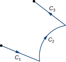
The next theorem summarizes several key properties of vector line integrals.
Let \(\vecs F\) and \(\vecs G\) be continuous vector fields with domains that include the oriented smooth curve \(C\). Then
- \(\displaystyle \int_C(\vecs F+\vecs G)·d\vecs{r}=\int_C \vecs{F} \cdot d\vecs{r}+\int_C \vecs G·d\vecs{r}\)
- \(\displaystyle \int_C k\vecs{F} \cdot d\vecs{r}=k\int_C \vecs{F} \cdot d\vecs{r}\), where \(k\) is a constant
- \(\displaystyle \int_{-C} \vecs{F} \cdot d\vecs{r}=-\int_{C}\vecs{F} \cdot d\vecs{r}\)
- Suppose instead that \(C\) is a piecewise smooth curve in the domains of \(\vecs F\) and \(\vecs G\), where \(C=C_1+C_2+⋯+C_n\) and \(C_1,C_2,…,C_n\) are smooth curves such that the endpoint of \(C_i\) is the starting point of \(C_{i+1}\). Then
\[\int_C \vecs F·d\vecs{r}=\int_{C_1} \vecs F·d\vecs{r}+\int_{C_2} \vecs F·d\vecs{r}+⋯+\int_{C_n} \vecs F·d\vecs{r} \nonumber \]
Notice the similarities between these items and the properties of single-variable integrals. Properties 1 and 2 say that line integrals are linear, which is true of single-variable integrals as well. Property 3 says that reversing the orientation of a curve changes the sign of the integral. If we think of the integral as computing the work done on a particle traveling along \(C\), then this makes sense. If the particle moves backward rather than forward, then the value of the work done has the opposite sign. This is analogous to the equation \(\displaystyle \int_a^b f(x)\,dx=−\int_b^af(x)\,dx\). Finally, if \([a_1,a_2]\), \([a_2,a_3]\),…, \([a_{n−1},a_n]\) are intervals, then
\[\int_{a_1}^{a_n}f(x) \,dx=\int_{a_1}^{a_2}f(x)\,dx+\int_{a_2}^{a_3}f(x)\,dx+⋯+\int_{a_{n−1}}^{a_n} f(x)\,dx, \nonumber \]
which is analogous to Property 4.
We will find \(\displaystyle \int_C (x-2y)\, dx+(y-x)\, dy\), where \(C\) is the rectangle (oriented counterclockwise) in a plane with vertices \((0,0)\), \((2,0)\), \((2,1)\), and \((0,1)\)
Note that curve \(C\) is the union of its four sides, and each side is smooth. Therefore \(C\) is piecewise smooth. Let \(C_1\) represent the side from \((0,0)\) to \((2,0)\), let \(C_2\) represent the side from \((2,0)\) to \((2,1)\), let \(C_3\) represent the side from \((2,1)\) to \((0,1)\), and let \(C_4\) represent the side from \((0,1)\) to \((0,0)\).
We graph \(\vecs{F}=\langle x-2y, y-x\rangle\) and \(C\):
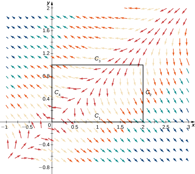
\[\int_C \vecs{F}\cdot d\vecs{r} =\int_{C_1} \vecs{F}\cdot d\vecs{r}+\int_{C_2} \vecs{F}\cdot d\vecs{r}+\int_{C_3} \vecs{F}\cdot d\vecs{r}+\int_{C_4} \vecs{F}\cdot d\vecs{r} \nonumber \]
We want to compute each of the four integrals on the right-hand side separately, so we need a parameterization of each side of the rectangle. Here are four parameterizations (note that they traverse \(C\) counterclockwise):
\[\begin{align*} C_1&:\,\vecs{r}_1(t)= ⟨t,0⟩,\quad \text{ for} \quad 0≤t≤2\\[4pt] C_2&:\,\vecs{r}_2(t)= ⟨2,t⟩,\quad \text{ for} \quad 0≤t≤1 \\[4pt] C_3&:\,\vecs{r}_3(t)= ⟨2−t,1⟩,\quad \text{ for} \quad 0≤t≤2\\[4pt] C_4&: \,\vecs{r}_4(t)=⟨0,1−t⟩,\quad \text{ for} \quad 0≤t≤1 \end{align*}\]
Therefore,
\[\begin{align*} \int_{C_1}\vecs{F}\cdot d\vecs{r} &=\int_0^2 ⟨t−2(0),0−t⟩·⟨1,0⟩ \,dt=\int_0^2 t \,dt =\Big[\dfrac{1}{2}t^2 \Big|_0^2=2 \\[8pt] \int_{C_2} \vecs{F} \cdot d\vecs{r} &=\int_{0}^{1}⟨2−2t,t−2⟩·⟨0,1⟩ \,dt=\int_{0}^{1} (t−2) \,dt =\Big[\dfrac{1}{2}t^2 −2t\Big|_0^1=−\dfrac{3}{2} \\[8pt]
\int_{C_3}\vecs{F}\cdot d\vecs{r}&=\int_0^2⟨(2−t)−2,1−(2−t)⟩·⟨−1,0⟩ \,dt =\int_0^2t \,dt=\left[ \dfrac{1}{2}t^2\right|_0^2 =2 \\[8pt]
\int_{C_4} \vecs{F}\cdot d\vecs{r}&=\int_0^1⟨−2(1−t),1−t⟩·⟨0,−1⟩ \,dt =\int_0^1(t−1) \,dt =\Big[\dfrac{1}{2}t^2 −t\Big|_0^1=−\dfrac{1}{2} \end{align*} \]
Thus, we have \(\displaystyle \int_C \vecs{F} \cdot d\vecs{r}=2+\left(-\dfrac{3}{2}\right)+2+\left(-\dfrac{1}{2}\right)=2\)
This page titled 3.5: Line Integrals was last modified on Thu, 16 Apr 2026 12:01:22 GMT and is shared under a CC BY-NC 4.0 license and was authored, remixed, and/or curated by Kenn Huber via source content that was edited to the style and standards of the LibreTexts platform.
The book could not be loaded just now.