Opening the book…
Our first step in studying the calculus of vector-valued functions is to define what exactly a vector-valued function is. We can then look at graphs of vector-valued functions and see how they define curves in both two and three dimensions.
A vector-valued function is a function of the form
\[\vecs r(t)=f(t)\,\hat{\mathbf{i}}+g(t)\,\hat{\mathbf{j}} \; \; \text{or} \; \;\vecs r(t)=f(t)\,\hat{\mathbf{i}}+g(t)\,\hat{\mathbf{j}}+h(t)\,\hat{\mathbf{k}} \nonumber \]
where the component functions \(f\), \(g\), and \(h\) are real-valued functions of the parameter \(t\). Vector-valued functions are also written in the form
\[\vecs r(t)=⟨f(t),\,g(t)⟩ \; \; \text{or} \; \; \vecs r(t)=⟨f(t),\,g(t),\,h(t)⟩ \nonumber \]
In both cases, the first form of the function defines a two-dimensional vector-valued function; the second form describes a three-dimensional vector-valued function. The parameter \(t\) might take on all real numbers or \(t\) can lie between two real numbers: \(a≤t≤b\). Last, the component functions themselves may have domain restrictions that enforce restrictions on the value of \(t\). We often use \(t\) as a parameter because \(t\) can represent time.
For each of the following vector-valued functions, evaluate \(\vecs r(0)\), \(\vecs r\left(\dfrac{\pi}{2}\right)\), and\(\vecs r\left(\dfrac{2\pi}{3}\right)\). Do any of these functions have domain restrictions?
(a) \(\vecs r(t)=4\cos( t)\,\hat{\mathbf{i}}+3\sin (t)\,\hat{\mathbf{j}}\)
(b) \(\vecs r(t)=3\tan( t)\,\hat{\mathbf{i}}+4 \sec( t)\,\hat{\mathbf{j}}+5t\,\hat{\mathbf{k}}\)
(a) To calculate each of the function values, substitute the appropriate value of \(t\) into the function:
\[ \begin{align*}\vecs r(0) = 4\cos(0) \hat{\mathbf{i}}+3\sin(0) \hat{\mathbf{j}}=4\hat{\mathbf{i}}+0 \hat{\mathbf{j}}=4\hat{\mathbf{i}} \\[4pt] \vecs r\left(\dfrac{\pi}{2}\right) = 4\cos\left(\dfrac{π}{2}\right)\hat{\mathbf{i}}+3\sin\left(\dfrac{π}{2}\right) \hat{\mathbf{j}}= 0\hat{\mathbf{i}}+3 \hat{\mathbf{j}}=3 \hat{\mathbf{j}} \\[4pt] \vecs r\left(\dfrac{2\pi}{3}\right) =4\cos\left(\dfrac{2π}{3}\right)\hat{\mathbf{i}}+3\sin\left(\dfrac{2π}{3}\right) \hat{\mathbf{j}} =4\left(−\dfrac{1}{2}\right)\hat{\mathbf{i}}+3\left(\dfrac{\sqrt{3}}{2}\right) \hat{\mathbf{j}}=−2 \hat{\mathbf{i}}+\dfrac{3 \sqrt{3}}{2} \hat{\mathbf{j}}\end{align*} \]
To determine whether this function has any domain restrictions, consider the component functions separately. The first component function is \(f(t)=4 \cos (t)\) and the second component function is \(g(t)=3\sin( t)\). Neither of these functions has a domain restriction, so the domain of \(\vecs r(t)=4\cos (t)\,\hat{\mathbf{i}}+3 \sin (t) \,\hat{\mathbf{j}}\) is all real numbers.
(b) To calculate each of the function values, substitute the appropriate value of t into the function:
\[\begin{align*}\vecs r(0) = 3\tan(0)\hat{\mathbf{i}}+4\sec(0) \hat{\mathbf{j}}+5(0) \hat{\mathbf{k}} = 0\hat{\mathbf{i}}+4j+0 \hat{\mathbf{k}}=4 \hat{\mathbf{j}} \\[4pt] \vecs r\left(\dfrac{\pi}{2}\right) = 3\tan\left(\dfrac{\pi}{2}\right)\hat{\mathbf{i}}+4\sec\left(\dfrac{\pi}{2}\right) \hat{\mathbf{j}}+5\left(\dfrac{\pi}{2}\right) \hat{\mathbf{k}} \text{ which does not exist} \\[4pt] \vecs r\left(\dfrac{2\pi}{3}\right) =3\tan\left(\dfrac{2 \pi}{3}\right)\hat{\mathbf{i}}+4\sec\left(\dfrac{2\pi}{3}\right) \hat{\mathbf{j}}+5\left(\dfrac{2\pi}{ 3}\right) \hat{\mathbf{k}} =3(−\sqrt{3})\hat{\mathbf{i}}+4(−2)\hat{\mathbf{j}}+\dfrac{10π}{3} \hat{\mathbf{k}} =(-3\sqrt{3})\hat{\mathbf{i}}−8\hat{\mathbf{j}}+\dfrac{10π}{3} \hat{\mathbf{k}}\end{align*}\]
To determine whether this function has any domain restrictions, consider the component functions separately. The first component function is \(f(t)=3\tan (t)\), the second component function is \(g(t)=4\sec (t)\), and the third component function is \(h(t)=5t\). The first two functions are not defined for odd multiples of \(\dfrac{\pi}{2}\), so the function is not defined for odd multiples of \(\dfrac{\pi}{2}\). Therefore, \[\text{D}_{\vecs r}=\Big\{t\,:\,t≠ \frac{(2n+1)\pi}{2}\Big\}\nonumber \] where \(n\) is any integer.
The domain of a vector-valued function consists of real numbers. The domain can be all real numbers or a subset of the real numbers. The range of a vector-valued function consists of vectors. Each real number in the domain of a vector-valued function is mapped to either a two- or a three-dimensional vector.
Recall that a plane vector consists of two quantities: direction and magnitude. Given any point in the plane (the initial point), if we move in a specific direction for a specific distance, we arrive at a second point (the terminal point). We calculate the components of the vector by subtracting the coordinates of the initial point from the coordinates of the terminal point.
A vector is considered to be in standard position if the initial point is located at the origin. When graphing a vector-valued function, we typically graph the vectors in the domain of the function in standard position, because doing so guarantees the uniqueness of the graph. This convention applies to the graphs of three-dimensional vector-valued functions as well. The graph of a vector-valued function of the form
\[\vecs r(t)=f(t)\, \hat{\mathbf{i}}+g(t)\,\hat{\mathbf{j}} \nonumber \]
consists of the set of all points \((f(t),\,g(t))\), and the path it traces is called a plane curve. The graph of a vector-valued function of the form
\[\vecs r(t)=f(t) \,\hat{\mathbf{i}}+g(t) \,\hat{\mathbf{j}}+h(t) \,\hat{\mathbf{k}} \nonumber \]
consists of the set of all points \((f(t),\,g(t),\,h(t))\), and the path it traces is called a space curve. Any representation of a plane curve or space curve using a vector-valued function is called a vector parameterization of the curve.
Each plane curve and space curve has an orientation, indicated by arrows drawn on the curve, that shows the direction of motion along the curve as the value of the parameter \(t\) increases.
Create a graph of each of the following vector-valued functions:
(a) The plane curve represented by \(\vecs r(t)=4 \cos( t) \,\hat{\mathbf{i}}+3 \sin (t) \,\hat{\mathbf{j}}\), \(0≤t≤2\pi\)
(b) The plane curve represented by \(\vecs r(t)=4 \cos(t^3) \,\hat{\mathbf{i}}+3 \sin(t^3) \,\hat{\mathbf{j}}\), \(0≤t≤\sqrt[3]{2\pi}\)
(c) The space curve represented by \(\vecs r(t)=4 \cos (t) \,\hat{\mathbf{i}}+4 \sin (t) \,\hat{\mathbf{j}}+t \,\hat{\mathbf{k}}\), \(0≤t≤4\pi\)
(a) As with any graph, we start with a table of values. We then graph each of the vectors in the second column of the table in standard position and connect the terminal points of each vector to form a curve.
| \(t\) | \(\vecs r(t)\) |
|---|---|
| \(0\) | \(4\hat{\mathbf{i}}\) |
| \(\dfrac{\pi}{4}\) | \(2 \sqrt{2} \hat{\mathbf{i}} + \dfrac{3 \sqrt{2}}{2}\hat{\mathbf{j}}\) |
| \(\dfrac{\pi}{2}\) | \(\mathrm{3\hat{\mathbf{j}}}\) |
| \(\dfrac{3\pi}{4}\) | \( -2 \sqrt{2} \hat{\mathbf{i}} + \dfrac{3 \sqrt{2}}{2}\hat{\mathbf{j}}\) |
| \(\pi\) | \(-4\hat{\mathbf{i}}\) |
| \(\dfrac{5\pi}{4}\) | \(-2 \sqrt{2} \hat{\mathbf{i}} - \dfrac{3 \sqrt{2}}{2}\hat{\mathbf{j}}\) |
| \(\dfrac{3\pi}{2}\) | \(\mathrm{-3\hat{\mathbf{j}}}\) |
| \(\dfrac{7\pi}{4}\) | \( 2 \sqrt{2} \hat{\mathbf{i}} - \dfrac{3 \sqrt{2}}{2}\hat{\mathbf{j}}\) |
| \(2\pi\) | \(4\hat{\mathbf{i}}\) |
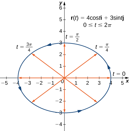
This curve travels counterclockwise along the ellipse \(\dfrac{x^2}{4^2}+\dfrac{y^2}{3^2}=1\).
(b) The table of values for \(\vecs r(t)=4 \cos(t^3) \,\hat{\mathbf{i}}+3 \sin(t^3) \,\hat{\mathbf{j}}\), for \(0≤t≤\sqrt[3]{2\pi}\) is as follows:
| \(t\) | \(\vecs r(t)\) |
|---|---|
| \(0\) | \(4\hat{\mathbf{i}}\) |
| \(\displaystyle \sqrt[3]{\dfrac{\pi}{4}}\) | \(2 \sqrt{2} \hat{\mathbf{i}} + \dfrac{3 \sqrt{2}}{2}\hat{\mathbf{j}}\) |
| \(\displaystyle \sqrt[3]{\dfrac{\pi}{2}}\) | \(\mathrm{3\hat{\mathbf{j}}}\) |
| \(\displaystyle \sqrt[3]{\dfrac{3\pi}{4}}\) | \( -2 \sqrt{2} \hat{\mathbf{i}} + \dfrac{3 \sqrt{2}}{2}\hat{\mathbf{j}}\) |
| \(\displaystyle\sqrt[3]{\pi}\) | \(-4\hat{\mathbf{i}}\) |
| \(\displaystyle \sqrt[3]{\dfrac{5\pi}{4}}\) | \(-2 \sqrt{2} \hat{\mathbf{i}} - \dfrac{3 \sqrt{2}}{2}\hat{\mathbf{j}}\) |
| \(\displaystyle \sqrt[3]{\dfrac{3\pi}{2}}\) | \(\mathrm{-3\hat{\mathbf{j}}}\) |
| \(\displaystyle \sqrt[3]{\dfrac{7\pi}{4}}\) | \( 2 \sqrt{2} \hat{\mathbf{i}} - \dfrac{3 \sqrt{2}}{2}\hat{\mathbf{j}}\) |
| \( \displaystyle\sqrt[3]{2\pi}\) | \(4\hat{\mathbf{i}}\) |
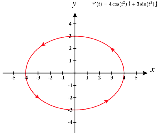
The graph of this curve is the same ellipse, it just does not travel around it at a constant "speed" as it did in part (a)
(c) We go through the same procedure for a three-dimensional vector function.
| \(t\) | \(\vecs r(t)\) |
|---|---|
| \(\mathrm{0}\) | \(\mathrm{4\hat{\mathbf{i}}}\) |
| \(\dfrac{\pi}{4}\) | \(\mathrm{2 \sqrt{2} \hat{\mathbf{i}} + 2\sqrt{2} \hat{\mathbf{j}} + \dfrac{\pi}{4} \hat{\mathbf{k}}}\) |
| \(\dfrac{\pi}{2}\) | \(\mathrm{4\hat{\mathbf{j}} +\dfrac{\pi}{2} \hat{\mathbf{k}}}\) |
| \(\dfrac{3\pi}{4}\) | \(\mathrm{ -2 \sqrt{2} \hat{\mathbf{i}} + 2\sqrt{2} \hat{\mathbf{j}} + \dfrac{3\pi}{4} \hat{\mathbf{k}}}\) |
| \(\mathrm{\pi}\) | \(\mathrm{-4\hat{\mathbf{i}}}+ \pi \hat{\mathbf{k}}\) |
| \(\dfrac{5\pi}{4}\) | \(\mathrm{ -2 \sqrt{2} \hat{\mathbf{i}} - 2\sqrt{2} \hat{\mathbf{j}} + \dfrac{5\pi}{4} \hat{\mathbf{k}}}\) |
| \(\dfrac{3\pi}{2}\) | \(\mathrm{-4\hat{\mathbf{j}} +\dfrac{3\pi}{2} \hat{\mathbf{k}}}\) |
| \(\dfrac{7\pi}{4}\) | \(\mathrm{ 2 \sqrt{2} \hat{\mathbf{i}} - 2\sqrt{2} \hat{\mathbf{j}} + \dfrac{7\pi}{4} \hat{\mathbf{k}}}\) |
| \(\mathrm{2\pi}\) | \(\mathrm{4\hat{\mathbf{i}} + 2\pi \hat{\mathbf{k}}}\) |
| \(\dfrac{9\pi}{4}\) | \(\mathrm{2 \sqrt{2} \hat{\mathbf{i}} + 2\sqrt{2} \hat{\mathbf{j}} + \dfrac{9\pi}{4} \hat{\mathbf{k}}}\) |
| \(\dfrac{5\pi}{2}\) | \(\mathrm{4\hat{\mathbf{j}} +\dfrac{5\pi}{2} \hat{\mathbf{k}}}\) |
| \(\dfrac{11\pi}{4}\) | \(\mathrm{ -2 \sqrt{2} \hat{\mathbf{i}} + 2\sqrt{2} \hat{\mathbf{j}} + \dfrac{11\pi}{4} \hat{\mathbf{k}}}\) |
| \(\mathrm{3\pi}\) | \(\mathrm{-4\hat{\mathbf{i}}}+ 3\pi \hat{\mathbf{k}}\) |
| \(\dfrac{13\pi}{4}\) | \(\mathrm{ -2 \sqrt{2} \hat{\mathbf{i}} - 2\sqrt{2} \hat{\mathbf{j}} + \dfrac{13\pi}{4} \hat{\mathbf{k}}}\) |
| \(\dfrac{7\pi}{2}\) | \(\mathrm{-4\hat{\mathbf{j}} +\dfrac{7\pi}{2} \hat{\mathbf{k}}}\) |
| \(\dfrac{15\pi}{4}\) | \(\mathrm{ 2 \sqrt{2} \hat{\mathbf{i}} - 2\sqrt{2} \hat{\mathbf{j}} + \dfrac{15\pi}{4} \hat{\mathbf{k}}}\) |
| \(\mathrm{4\pi}\) | \(\mathrm{4\hat{\mathbf{i}} + 4\pi \hat{\mathbf{k}}}\) |
The values then repeat themselves, except for the fact that the coefficient of \(\hat{\mathbf{k}}\) is always increasing.
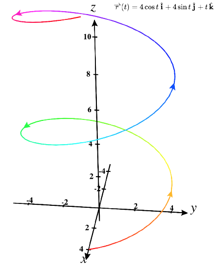
This curve is called a helix. Notice that if the \(\hat{\mathbf{k}}\) component is eliminated, then the function becomes \(\vecs r(t)=4\cos (t) \hat{\mathbf{i}}+ 4\sin (t) \hat{\mathbf{j}}\), which is a circle of radius 4 centered at the origin. That circle is exactly what the view of this space curve would look like if you were looking down from above.
You may notice that the graphs in parts (a) and (b) are identical. This happens because the function describing the curve in part (b) is a so-called reparameterization of the function describing the curve in part (a). In fact, any curve has an infinite number of reparameterizations; for example, we can replace \(t\) with \(2t\) in any of the three previous curves without changing the shape of the curve. The interval over which \(t\) is defined may change, but that is all. We return to this idea later when we study arc-length parameterization.
As mentioned, the name of the shape of the curve of the graph is a helix. The curve resembles a spring, with a circular cross-section looking down along the \(z\)-axis. The arrows in the graph of this helix indicate the orientation of the curve as \(t\) progresses from \(0\) to \(4π\). It is possible for a helix to be elliptical in cross-section as well. For example, the vector-valued function \(\vecs r(t)=4 \cos (t) \,\hat{\mathbf{i}}+3 \sin (t) \,\hat{\mathbf{j}}+t \,\hat{\mathbf{k}}\) describes an elliptical helix. The projection of this helix into the \(xy\)-plane is an ellipse. If you consider each component function parametrically:
\[ \left\{ \begin{array} {l} x(t)=4\cos(t) \\ y(t)=3\sin(t) \\ z(t)=t \end{array} \right. \longrightarrow \cos(t)=\dfrac{x}{4} \text{ and } \sin(t)= \dfrac{y}{3} \nonumber\]
Since we know \(\cos^2(t)+\sin^2(t)=1\) always holds, we see that this space curve must lie on the cylinder \(\left(\dfrac{x}{4}\right)^2+\left(\dfrac{y}{3}\right)^2=1\). We see that \(z\) moves linearly at the same rate that \(t\) increases the angle inside of cosine and sine, which is why our spring is evenly spaced and counterclockwise along this cylinder. We can use our knowledge of previous sections to more easily visualize space curves.
Use different coordinate systems to help sketch each vector valued curve.
(a) \(\vecs r(t)=(2+\sin(t)) \cos(t) \,\hat{\mathbf{i}}+(2+\sin(t)) \sin(t) \,\hat{\mathbf{j}}\), for \(0≤t≤2\pi\)
(b) \(\vecs r(t)=t\cos(t) \,\hat{\mathbf{i}}+t \sin(t) \,\hat{\mathbf{j}}+t \,\hat{\mathbf{k}}\), \(0≤t≤ 4\pi\)
(c) \(\vecs r(t)=t\cos(t) \,\hat{\mathbf{i}}+t \sin(t) \,\hat{\mathbf{j}}+2t^2 \,\hat{\mathbf{k}}\), \(0≤t≤ 2\pi\)
(d) \(\vecs r(t)=\sin(t)\cos(4t) \,\hat{\mathbf{i}}+ \sin(t)\sin(4t) \,\hat{\mathbf{j}}+\cos(t) \,\hat{\mathbf{k}}\), \(0≤t≤ \pi\)
(a) Notice that this curve looks better in polar form:
\[\vecs r(t)=R(t)\cos(\theta (t))\hat{\mathbf{i}}+R(t) \sin(\theta(t)) \,\hat{\mathbf{j}} \longleftrightarrow R(t)=2+\sin(t) \text{ and } \theta(t)=t\nonumber \]
Since \(t=\theta\), this is just the polar graph \(R=2+\sin(\theta)\) traversed in the standard counterclockwise direction:

(b) This space curve is nicer in cylindrical form:
\[\vecs r(t)=R(t)\cos(\theta(t))\hat{\mathbf{i}}+R(t) \sin(\theta(t)) \,\hat{\mathbf{j}}+z(t) \,\hat{\mathbf{k}} \longleftrightarrow R(t)=t \text{ and } \theta(t)=t \text{ and } z(t)=t \nonumber \]
Since \(R=t\), this is the cylindrical relationship \(R=\theta\) and \(z=R \). Note that \(z=R\) in cylindrical coordinates is a cone, so we will spiral outward around the surface of this cone in the standard counterclockwise direction while \(z\) climbs upward at the same rate we rotate.

(c) This space curve is also nicer in cylindrical form:
\[\vecs r(t)=R(t)\cos(\theta(t))\hat{\mathbf{i}}+R(t) \sin(\theta(t)) \,\hat{\mathbf{j}}+z(t) \,\hat{\mathbf{k}} \longleftrightarrow R(t)=t \text{ and } \theta(t)=t \text{ and } z(t)=2t^2 \nonumber \]
Since \(R=t\), this is the cylindrical relationship \(R=\theta\) and \(z=2R^2\). Note that \(z=2R^2\) in cylindrical coordinates is a paraboloid, so we will travel around the surface of this paraboloid in the standard counterclockwise direction while \(z\) climbs upward at increasing speeds as we rotate.

(d) This space curve is nicer in spherical form:
\[\vecs r(t)=\rho(t)\sin(\phi(t))\cos(\theta(t) )\hat{\mathbf{i}}+\rho(t)\sin(\phi(t)) \sin(\theta(t)) \,\hat{\mathbf{j}}+\rho(t)\cos(\phi(t)) \,\hat{\mathbf{k}} \longleftrightarrow \rho(t)=1 \text{ and } \phi(t)=t \text{ and } \theta(t)=4t \nonumber \]
Since \(\rho=1\) is constant, we know this curve travels along the surface of the unit sphere. We have the spherical relationship \(\theta=4\phi \), so we will travel around the surface of this sphere from the top downward and make 2 full counterclockwise rotations in the theta direction.

We can also approach these types of problems in reverse when asked to parameterize the intersections of surfaces.
Find a parameterization of the intersection of the surfaces provided.
(a) \(x^2+y^2+z^2=2\) and \(x=y^2+z^2\)
(b) \(3x^2+y^2+z^2=1\) and \(x+z=0\)
(c) \( z=x^2-y^2\) and \(\dfrac{x^2}{16}+\dfrac{y^2}{4}=1\)
(a) First we sketch the intersection of the sphere \(x^2+y^2+z^2=2\) and the paraboloid \(x=y^2+z^2\):

We can substitute the paraboloid equation into the sphere to get \( x^2+x=2\) which has solutions \(x=-2,1\)
Since \(x=-2\) is impossible on the paraboloid, we must have \(x(t)=1\) for all \(t\).
Now we want \(1=(y(t))^2+(z(t))^2\), which we can parameterize with \(y(t)=\sin(t),z(t)=\cos(t)\) for \(0≤t≤ 2\pi\)
Therefore we have \(\vecs r(t) =1 \,\hat{\mathbf{i}}+ \sin(t) \,\hat{\mathbf{j}}+\cos(t) \,\hat{\mathbf{k}}\) with \(0≤t≤ 2\pi\)
(Note that \(\vecs r(t) =1 \,\hat{\mathbf{i}}+ \cos(t) \,\hat{\mathbf{j}}+\sin(t) \,\hat{\mathbf{k}}\) would also work)
(b) We sketch the intersection of the ellipsoid \(3 x^2 +y^2 +z^2=1\) and the plane \(x+z=0\):

We substitute the plane \(z=-x\) into the ellipsoid to get \(3 x^2 +y^2 +(-x)^2=1\)
This simplifies to \(4x^2+y^2=1\) which is an ellipse. We pick \(x(t)\) and \(y(t)\) so that \(4((x(t))^2+(y(t))^2=1\)
One such possibility is \(x(t)=\dfrac{1}{2}\cos(t)\) and \(y(t)=\sin(t)\) with \(0≤t≤ 2\pi\)
Since \(z=-x\) we must then have \(z(t)=-\dfrac{1}{2}\cos(t)\)
Therefore we have \(\vecs r(t) =\dfrac{1}{2}\cos(t)\,\hat{\mathbf{i}}+ \sin(t) \,\hat{\mathbf{j}}-\dfrac{1}{2}\cos(t) \,\hat{\mathbf{k}}\) with \(0≤t≤ 2\pi\)
(c) Again we sketch the intersection of the hyperbolic paraboloid \( z=x^2-y^2\) and cylinder \(\dfrac{x^2}{16}+\dfrac{y^2}{4}=1\):

Luckily, the cylinder already has only two variables, so we can parameterize \(x(t)\) and \(y(t)\) along its edge.
One possibility is to pick \(x(t)=4\cos(t)\) and \(y(t)=2\sin(t)\) with \(0≤t≤ 2\pi\)
Since \(z=x^2-y^2\), we have \(z(t)=(4\cos(t))^2-(2\sin(t))^2=16\cos^2(t)-4\sin^2(t)\)
Therefore we have \(\vecs r(t)=4\cos(t)\,\hat{\mathbf{i}}+ 2\sin(t) \,\hat{\mathbf{j}}+\left(16\cos^2(t)-4\sin^2(t)\right) \,\hat{\mathbf{k}}\) with \(0≤t≤ 2\pi\)
At this point, you may notice a similarity between vector-valued functions and parameterized curves. Indeed, given a vector-valued function \(\vecs r(t)=f(t)\,\hat{\mathbf{i}}+g(t)\,\hat{\mathbf{j}}\) we can define \(x=f(t)\) and \(y=g(t)\). If a restriction exists on the values of \(t\) (for example, \(t\) is restricted to the interval \([a,b]\) for some constants \(a<b\)), then this restriction is enforced on the parameter. The graph of the parameterized function would then agree with the graph of the vector-valued function, except that the vector-valued graph would represent vectors rather than points. Since we can parameterize a curve defined by a function \(y=f(x)\), it is also possible to represent an arbitrary plane curve by a vector-valued function. Just use \(\vecs{r}(t)=t \,\hat{\mathbf{i}}+ f(t)\,\hat{\mathbf{j}}\)
This page titled 1.6: Vector-Valued Functions was last modified on Tue, 14 Apr 2026 23:21:16 GMT and is shared under a CC BY-NC 4.0 license and was authored, remixed, and/or curated by Kenn Huber via source content that was edited to the style and standards of the LibreTexts platform.
The book could not be loaded just now.