Opening the book…
- Note to the Instructor (click to expand)
- I chose to only introduce the graphs of the sine, cosine, and tangent because these are the foundational graphs for the remainder of trigonometry. The graphs of the remaining trigonometric functions are held off until the very end of the chapter. Additionally, this section introduces the symmetry of these functions. Therefore, we can spend some time doing proofs involving symmetry and these functions.
- (click to expand)
-
- Sets and Numbers
- Rational Functions
The following is a list of learning objectives for this section.
- Learning Objectives (click to expand)
-
- Sketch the base graphs of the fundamental trigonometric functions.
- Determine whether the graph of an equation involving trigonometric functions is even, odd, or neither.
- Evaluate a trigonometric function using the Symmetry Identities.
When you were learning Algebra, you were introduced to variables, expressions involving variables, equations involving variables, and graphs of those equations (in that order). In Trigonometry, this order is slightly modified. We have learned about trigonometric functions and manipulated expressions involving those functions; however, before solving equations involving those functions, it's best to be able to visualize their graphs.
This section focuses on the base graphs of the fundamental trigonometric functions.
The graphs of the remaining trigonometric functions will be introduced after we have a few sections to get used to the graphs of the fundamental trigonometric functions.
Motivating Periodic Functions of Angles
Imagine that you are riding on a Ferris wheel. As the wheel turns, your height above the ground increases and decreases. This pattern repeats each time the Ferris wheel makes a complete rotation. This type of motion is called periodic motion.
In Mathematics, we seek to model periodic motion with a function.
We use periodic functions to model phenomena that exhibit cyclical behavior, such as the height of tides, seasonal growth patterns in plants and animals, radio waves, and planetary motion.
Let's create a mathematical model for a ride on a Ferris wheel. Suppose the Ferris wheel has a radius of 100 feet and rotates counterclockwise. Our model will be a function that describes the rider's height above the ground as they ride the wheel. To graph the Ferris wheel function, we must first specify the input and output variables and then choose a coordinate system to display their values.
While developing the model, let's place the origin at the center of the Ferris wheel (see Figure \(\PageIndex{1}\) below).

While this is not the most realistic placement for us to imagine (it makes us think that the bottom of the Ferris wheel is below ground level), this temporary placement will reveal an important characteristic of the rider's motion. The line from the origin to the rider's position on the wheel makes an angle, \( \theta \), with the horizontal. This angle will be the independent variable for the function. The height of the rider, \(h\), is also a variable and is related to the \(y\)-coordinate of the rider's position. Figure \(\PageIndex{1}\) shows that \(h = y + 100\) because the center of the wheel is 100 feet above the ground.
Let's focus on the rider's height as a function of angle. Therefore, we'll first graph \(y\) as the dependent variable instead of \(h\). As the angle \(\theta\) increases from \(0^{\circ}\) to \(90^{\circ}\), the rider's \(y\)-coordinate increases from 0 to 100. At that point, they are at the top of the wheel. Then, as \(\theta\) increases from \(90^{\circ}\) to \(180^{\circ}\), the rider's \(y\)-coordinate decreases from 100 back to 0 (see Figure \(\PageIndex{2}\)).

Finally, as \(\theta\) increases from \(180^{\circ}\) to \(360^{\circ}\), the rider's \(y\)-coordinate decreases from 0 to -100 and then increases from -100 back to 0. At that point, the rider has made one complete rotation on the Ferris wheel. If she goes around again, \(\theta\) increases from \(360^{\circ}\) to \(720^{\circ}\), and the graph of her \(y\)-coordinate will repeat the pattern of the first rotation. Again, Figure \(\PageIndex{2}\) shows how the rider's \(y\)-coordinate is plotted as a function of the angle \(\theta\).
Look back at Figure \(\PageIndex{1}\) and notice from the reference triangle that \( \sin\left( \theta \right) = \frac{y}{100}\). Therefore, \(y = 100 \sin\left( \theta \right)\). For example, when \(\theta=30^{\circ}\), the \(y\)-coordinate of the rider is\[y=100 \sin \left(30^{\circ}\right)=100\left(\frac{1}{2}\right)=50\nonumber\]and the rider's height above the ground is \( h = y + 100 = 150 \, \text{feet} \). In general, then, \(h\) is given as a function of \(\theta\) by\[h=y+100=100 \sin \left(\theta\right)+100.\nonumber\]This is our model for a rider's height on a Ferris wheel as a function of angle.
The graph on the right side of Figure \(\PageIndex{2}\) is called a sine curve.
While it might seem odd that we use the blanket phrase "sine curve" when describing a graph derived from the sine or the cosine, this consolidation will make sense shortly.
An Aside: Degrees or Radians?
Before we go any further, we need to make one thing clear:
Figure \(\PageIndex{2}\) is the first and the last time you will see a graph of the sine (or any other trigonometric) function in terms of degrees.
While there are several reasons that we endeavor only to graph trigonometric functions using radians, the two most impactful are the relation to the unit circle and scale. When we derived the unit circle definition of the trigonometric functions, we did so using radian measure. If we redraw Figure \(\PageIndex{2}\) using radians as the angular measure (and the unit circle instead of a circle of radius 100), we get Figure \(\PageIndex{3}\).

Note that the scale on the vertical axis (namely, that the largest and smallest \( y \)-values are \( 1 \) and \( -1 \), respectively) and the scale on the horizontal axis (from \( x = 0 \) to \( x = 2\pi \)) are more closely aligned than had we kept the angular measure in degrees.
Graphing the Sine Function
There are two main ways students initially learn to graph the sine function—by plotting points or by tracing the \( y \)-values along the unit circle. The latter is what we did in Figure \(\PageIndex{3}\). The former is not the ideal method, but it's a good idea to showcase it right now so we can link the computed values of the sine function to points on a graph.
Point-Plotting Approach
Up to this point, we have mostly let sine be a function of the angle \( \theta \); however, we recently discovered (via our discussion of circular functions) that the trigonometric functions are also functions of real numbers. Therefore, we should feel fine working with \( f(x) = \sin\left( x \right) \). The independent variable, \( x \), could represent an angle, the arc length along a circle, or time—our application determines the context.
Sketch a portion of the graph of \( y = \sin\left( x \right) \) on the interval \( \left[ 0, 2\pi \right] \) by making a table of values.
- Solution
-
To graph \( f(x) = \sin\left( x \right) \) without relating to the unit circle, we need to list out several values of the sine function.\[\begin{array}{|c|c|c|c|c|c|c|c|c|c|} \hline x & 0 & \dfrac{\pi}{4} & \dfrac{\pi}{2} & \dfrac{3\pi}{4} & \pi & \dfrac{5\pi}{4} & \dfrac{3\pi}{2} & \dfrac{7\pi}{4} & 2\pi \\[6pt] \hline \sin\left( x \right) \, (\text{exact}) & 0 & \dfrac{1}{\sqrt{2}} & 1 & \dfrac{1}{\sqrt{2}} & 0 & -\dfrac{1}{\sqrt{2}} & -1 & -\dfrac{1}{\sqrt{2}} & 0 \\[6pt] \hline \sin\left( x \right) \, (\text{approximate}) & 0 & 0.707 & 1 & 0.707 & 0 & -0.707 & -1 & -0.707 & 0 \\[6pt] \hline \end{array}\nonumber\]Plotting these values and connecting them with a smooth curve, we get the following:

Figure \(\PageIndex{4}\)
Sketch a portion of the graph of \( y = \sin\left( x \right) \) on the interval \( \left[ -\frac{3\pi}{2}, \frac{\pi}{2} \right] \) by making a table of values.
- Answer
-

Figure \(\PageIndex{5}\)
There are several issues with plotting points to obtain the sine function graph. The first is the amount of time spent computing values. We will be graphing the sine curve throughout the rest of our mathematical journey, and if we need to plot points every time we graph, we will be wasting time and effort. The second issue has to do with "connecting the dots." Those who have no idea of the curvature of the sine graph end up connecting the points with lines and arrive at something like Figure \(\PageIndex{6}\).

I hope you can see the difference between the correct graph of the sine function from Example \(\PageIndex{1}\) and the incorrect graph represented in Figure \(\PageIndex{6}\).
The third issue with graphing using point-plotting involves building a natural understanding of the sine curve. Many features, like domain and range, slip out of the student's grasp, who consistently requires the "connect the dots" method when graphing trigonometric functions.
Finally, the fourth issue occurs when needing to extend the graph of the sine function beyond the interval \( \left[ 0, 2\pi \right] \). As Checkpoint \(\PageIndex{1}\) shows, and as we shall see in more concrete form shortly, the sine curve oscillates in both directions (as \( x \to \infty \) and as \( x \to - \infty \)). If we needed to plot points to extend the graph, we would be plotting and computing for a long time.
With all these considerations in mind, we will avoid using point-plotting when graphing trigonometric functions (other than introducing the base graphs of the trigonometric functions).
Unit Circle Approach
We have already motivated the sine curve using the unit circle in Figure \(\PageIndex{3}\); however, let's spend a few more moments solidifying our understanding of the relationship between the unit circle and the sine curve.
Recall, \( \sin\left( t \right) \) is the value of the \( y \)-coordinate for the point \( P \) on the unit circle, where \( t \) is simultaneously the arc length from \( \left( 1,0 \right) \) to the point \( P \) and the angle subtended by this arc. The following Interactive Element shows how the sine curve is created by tracing these \( y \)-coordinates as the angle (or arc length) \( t \) increases from \( 0 \) to \( 2\pi \) (if you only have access to the PDF of this textbook, then please go to the following link: https://www.desmos.com/calculator/aq5r4ka4dd)
Observation: As the angle (or arc length) \( t \) increases, the \( y \)-coordinate increases to \( 1 \), then decreases to \( -1 \), then increases back to \( y=0 \).
We now can easily "extend" the graph of the sine function by allowing \( t \) to go beyond \( 2\pi \) (https://www.desmos.com/calculator/imbgdopjtz).
Basic Features of the Sine Curve
Now that we know how to graph the base sine curve, we can dive into the details of this function.
Domain and Range
We now have enough knowledge to graph the entire sine curve. Figure \(\PageIndex{7}\) shows the general sine curve along with a single cycle (in blue) on the interval \( \left[ 0,2\pi \right] \).

Since the sine curve oscillates forever in both directions, it should be evident that the sine function has an output for every input. Therefore, the domain of the sine function is all real numbers. Moreover, we can see from the graph that the values of the sine function oscillate between \( -1 \) and \( 1 \) (inclusive). Hence, the range must be \( \left[ -1,1 \right] \). We summarize these results in the following theorem.
It is common for those learning Trigonometry to need clarification about the meaning of the argument of the sine function at this point. When we speak of the unit circle, we are speaking of the graph of all solutions, \( \left( x,y \right) \), to the equation\[x^2 + y^2 = 1.\nonumber\]As was mentioned in a previous section, the \( x \)-coordinate of a point on the unit circle is defined to be \( \cos\left( t \right) \) and the \( y \)-coordinate is defined to be \( \sin\left( t \right) \), where \( t \) is simultaneously the arc length along the unit circle to the point in question and the angle subtended by that arc length.
Unfortunately, we will now be graphing \( f(x) = \sin\left( x \right) \). This value of \( x \) differs from the related \( x \)-coordinate on the unit circle! You can (and should) think of the \( x \) in \( f(x) = \sin\left( x \right) \) as a "dummy variable." If you prefer to replace it with \( \theta \) or \( t \), please feel free to do so; however, we will continue to write sine as a function of \( x \) to get you used to this often confusing convention.
Period
Another observation is that the sine function repeats its pattern every \( 2\pi \) units along the \( x \)-axis.
If we take any interval of length \( 2\pi \) along the \( x \)-axis, we will see that the corresponding section of the sine curve over that interval can be "copied-and-pasted" an infinite number of times to create the entire sine curve. For example, while not convenient, we could consider the interval \( \left[ -5, -5 + 2\pi \right] \) along the \( x \)-axis, as shown in Figure \(\PageIndex{8}\) below.

"Copying-and-pasting" that segment an infinite number of times in both directions, we rebuild the entire sine curve.

Moreover, if we had selected a smaller interval along the \( x \)-axis, say \( \left[ -5,-5 + \frac{3\pi}{2} \right] \), we would not have captured enough of the behavior of the sine curve to appropriately recreate the entire curve by "copying-and-pasting" the smaller section.

Hence, by the definition of the period of a function, the following theorem should make sense.
While the graph of the sine function (and all of the other trigonometric functions) extends in both directions forever (see Figure \(\PageIndex{7}\)), the section of the graph starting at \( x = 0 \) and ending at \( x = 2\pi \) is going to be very important as we move forward.
Thus, by definition, we get the following theorem.
It is important to note that there are other periodic functions besides the sine function.
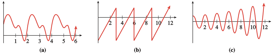
Which of the functions shown below are periodic? If the function is periodic, give its period.

- Solutions
-
- This graph is periodic with period 360.
- This graph is not periodic.
- This graph is periodic with period 8.
Which of the functions shown below are periodic? If the function is periodic, give its period.
- Answers
-
- Period: 2
- Period: 3
- Not periodic
A patient receives regular doses of medication to maintain a certain level of the drug in his body. After each dose, the patient's body eliminates a certain percentage of the medication before the next dose. The graph shows the amount of the drug, in milliliters, in the patient's body as a function of time in hours.

- How much of the medication is administered with each dose?
- How often is the medication administered?
- What percent of the drug is eliminated from the body between doses?
- Solutions
-
- The medication level increases from 30 ml to 50 ml at each cycle of the graph, so 20 ml of medication is administered at each dose.
- The medication level peaks sharply every four hours after administering each new dose.
- The medication level declines by \(20\) ml between doses, or \(\frac{20}{50} = 0.6\), or \(60\%\).
You are sitting on your front porch late one evening, and you see a light coming down the road tracing out the path shown below, with distances in inches. You realize you are seeing a bicycle light fixed on a bike's front wheel.
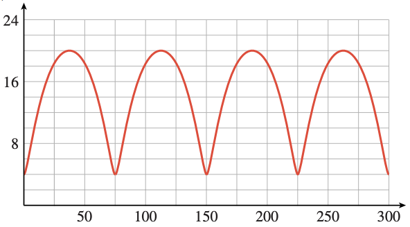
- Approximately what is the period of the graph?
- How far above the ground is the light?
- What is the diameter of the bicycle wheel?
- Answers
-
- 75 in
- 4 in
- 24 in
Amplitude
The sine curve (and, as we shall soon see, the cosine curve) has a feature almost exclusively unique among the graphs of all other functions—amplitude.
That is, the amplitude is half the distance between the highest and lowest values of the function.
Determine the amplitude of each function.
-

Figure \(\PageIndex{15}\) -

Figure \(\PageIndex{16}\)
- Solutions
-
- The maximum value for the graph of this function is \( M = 4 \) and the minimum is \( m = 2 \). Therefore, the amplitude of the graph is\[\text{Amplitude} = \dfrac{1}{2} \left| 4 - 2 \right| = 1.\nonumber\]
- The maximum value is \( M = 50 \) and the minimum is \( m = 30 \). Thus,\[\text{Amplitude} = \dfrac{1}{2} \left| 50 - 30 \right| = 10.\nonumber\]
Determine the amplitude and period of the function.

- Answer
-
Period: \( \pi \)
Amplitude: 2.5
The concept of amplitude is generally reserved for the sine and cosine functions; however, it occasionally gets referenced when working with other periodic functions.
Zeros
We know that the graph of \( f(x) = \sin\left( x \right) \) crosses the \( x \)-axis when \( \sin\left( x \right) = 0 \); however, using the intuitive visualization of the sine function being the \( y \)-coordinates of points along the edge of the unit circle, we can see (from Figure \(\PageIndex{3}\), Example \(\PageIndex{1}\), or either of the Interactive Elements above) that this occurs when \( x = 0, \pi, 2\pi, -\pi, -2\pi, \ldots \). The following theorem provides a much better way to write this.
As a reminder, the notation, \( \in \), means "belongs to" and the notation, \( \mathbb{Z} \), means "the set of all integers." Therefore, as long as \( k \in \mathbb{Z} \), \( x = \pi k \) is shorthand for\[x = 0, \pm \pi, \pm 2\pi, \pm 3\pi, \pm 4 \pi, \cdots.\nonumber\]We will be using this notation extensively from this point forward in Mathematics.
Graphing the Cosine Function
Now that we have set the foundation for all the concepts we need, our discussion of the cosine function graph will be shorter than that of the sine function. We begin using the worst method for graphing a function—point-plotting.
Point-Plotting Approach
Sketch a portion of the graph of \( y = \cos\left( x \right) \) on the interval \( \left[ 0, 2\pi \right] \) by making a table of values.
- Solution
-
\[\begin{array}{|c|c|c|c|c|c|c|c|c|c|} \hline x & 0 & \dfrac{\pi}{4} & \dfrac{\pi}{2} & \dfrac{3\pi}{4} & \pi & \dfrac{5\pi}{4} & \dfrac{3\pi}{2} & \dfrac{7\pi}{4} & 2\pi \\[6pt] \hline \cos\left( x \right) \, (\text{exact}) & 1 & \dfrac{1}{\sqrt{2}} & 0 & -\dfrac{1}{\sqrt{2}} & -1 & -\dfrac{1}{\sqrt{2}} & 0 & \dfrac{1}{\sqrt{2}} & 1 \\[6pt] \hline \cos\left( x \right) \, (\text{approximate}) & 1 & 0.707 & 0 & -0.707 & -1 & -0.707 & 0 & 0.707 & 1 \\[6pt] \hline \end{array}\nonumber\]Plotting these values and connecting them with a smooth curve, we get the following:

Figure \(\PageIndex{18}\)
Sketch a portion of the graph of \( y = \cos\left( x \right) \) on the interval \( \left[ -\frac{3\pi}{2}, \frac{\pi}{2} \right] \) by making a table of values.
- Answer
-

Figure \(\PageIndex{19}\)
Unit Circle Approach
Relating the cosine curve to the unit circle is similar to what we did with the sine curve; however, we must remember that \( \cos\left( t \right) \) is the \( x \)-coordinate of the points on the unit circle. This makes the visual a little more challenging, but you can play with the following Interactive Element (https://www.desmos.com/calculator/rr51fjmchw) to help cement the concept.
Observation: As the angle (or arc length) \( t \) increases, the \( x \)-coordinate decreases from \( 1 \) to \( -1 \), then increases from \( -1 \) back to \( 1 \).
As before, we show the general cosine curve along with a single cycle (in blue) on the interval \( \left[ 0,2\pi \right] \) in Figure \(\PageIndex{20}\) below.

It is no coincidence that the graph in Figure \(\PageIndex{20}\) has many characteristics resembling the graph of the sine function (Figure \(\PageIndex{7}\)). The sine and cosine functions are highly related, so their graphs are similar (but not the same). We will explore this similarity later.
Domain, Range, Period, Amplitude, and Zeros
As with the graph of the sine function, the graph of the cosine function reveals the domain and range of the cosine, its period, and the amplitude.
Finally, we know that the graph of \( f(x) = \cos\left( x \right) \) crosses the \( x \)-axis when \( \cos\left( x \right) = 0 \). This happens when the \( x \)-coordinates of points along the edge of the unit circle become \( 0 \). This occurs when the angular argument of the cosine function is \(\pm \frac{\pi}{2}\), \( \pm \frac{3\pi}{2}\), \( \pm \frac{5\pi}{2} \), \(\pm \frac{7\pi}{2} \), \(\ldots \). The following theorem summarizes this result.
There are other ways you could write this set of zeros. For example,\[x = \dfrac{\pi}{2} + \pi k = \dfrac{\pi}{2} + \dfrac{2\pi k}{2} = \dfrac{\pi + 2\pi k}{2} = \dfrac{\pi}{2} \left(1 + 2k\right) = \left( 2k + 1 \right) \dfrac{\pi}{2}.\nonumber\]I find that students remember the form given in the theorem the best.
Graphing the Tangent Function
The tangent function is the more abstract graph of the fundamental trigonometric functions. Therefore, we will spend much time deriving the graph and discussing how it is generated. In the end, students will gravitate to either the conceptual approach (which uses the graphs of the sine and cosine to help develop the tangent curve) or the unit circle approach (which uses the slope of the terminal side of the angle). Understanding both approaches to graphing the tangent curve is best because both will be needed in future mathematics courses.
Before we get to those "headier" approaches to graphing the tangent function, we start, as we did with the sine curve, by plotting points.
Point-Plotting Approach
As with the sine and cosine functions, we begin by making a table of values and plotting points. If we decide to use the same "test points" to build our table of values, something odd happens.\[\begin{array}{|c|c|c|c|c|c|c|c|c|c|} \hline x & 0 & \dfrac{\pi}{4} & \dfrac{\pi}{2} & \dfrac{3\pi}{4} & \pi & \dfrac{5\pi}{4} & \dfrac{3\pi}{2} & \dfrac{7\pi}{4} & 2\pi \\[6pt] \hline \tan\left( x \right) & 0 & 1 & \text{Undefined} & -1 & 0 & 1 & \text{Undefined} & -1 & 0 \\[6pt] \hline \end{array}\nonumber\]The fact that the tangent function is undefined at \( \frac{\pi}{2} \) and \( \frac{3\pi}{2} \) should not be surprising. By the Ratio Identity, \( \tan\left( x \right) = \frac{\sin\left( x \right)}{\cos\left( x \right)} \), and we have just mentioned that the cosine has zeros at \( x = \frac{\pi}{2} + \pi k \). That is, the tangent function encounters division by zero at \( x = \pm \frac{\pi}{2}, \pm \frac{3\pi}{2}, \pm \frac{5\pi}{2}, \ldots \).
What does this mean about the graph of the tangent function? If we decide to plot the points in our list where the tangent is defined, all we would get is the following graph.

We are now faced with the question, "How do we connect these points?"
This is one of the many weaknesses of graphing via point-plotting—we are often left guessing how the graph behaves between the points.
In these situations, most people plot more points to see if the true behavior of the graph reveals itself. If we make our table more robust by including every special angle from \( 0 \) to \( 2\pi \), we get the following:\[\begin{array}{|c|c|c|c|c|c|c|c|c|c|c|c|c|c|c|c|c|c|} \hline x & 0 & \dfrac{\pi}{6} & \dfrac{\pi}{4} & \dfrac{\pi}{3} & \dfrac{\pi}{2} & \dfrac{2\pi}{3} & \dfrac{3\pi}{4} & \dfrac{5\pi}{6} & \pi & \dfrac{7\pi}{6} & \dfrac{5\pi}{4} & \dfrac{4\pi}{3} & \dfrac{3\pi}{2} & \dfrac{5\pi}{3} & \dfrac{7\pi}{4} & \dfrac{11\pi}{6} & 2\pi \\[6pt] \hline \tan\left( x \right) \, (\text{exact}) & 0 & \dfrac{1}{\sqrt{3}} & 1 & \sqrt{3} & \text{Undefined} & -\sqrt{3} & -1 & -\dfrac{1}{\sqrt{3}} & 0 & \dfrac{1}{\sqrt{3}} & 1 & \sqrt{3} & \text{Undefined} & -\sqrt{3} & -1 & -\dfrac{1}{\sqrt{3}} & 0 \\[6pt] \hline \tan\left( x \right) \, (\text{approximate}) & 0 & 0.577 & 1 & 1.732 & \text{Undefined} & -1.732 & -1 & 0.577 & 0 & 0.577 & 1 & 1.732 & \text{Undefined} & -1.732 & -1 & 0.577 & 0 \\[6pt] \hline \end{array}\nonumber\]However, as detailed and exhaustive as this might seem, the graphical result is only slightly better.

While Figure \(\PageIndex{22}\) begins to reveal some of the patterns of the tangent graph, it's not quite revealing everything we need. Therefore, we must throw in the proverbial towel and try a different method of graphing the tangent function.
Unit Circle Approach
From the unit circle definition of the trigonometric functions, if \( P\left( x,y \right) \) is a point on the unit circle, then \( \tan\left( \theta \right) = \frac{y}{x} \), where \( \theta \) is the angle from the positive \( x \)-axis to the ray connecting the origin to \( P \) (see Figure \(\PageIndex{23}\)).

Therefore, \( \tan\left( \theta \right) \) is the slope of the ray connecting the origin to \( P \). When \( \theta = 0 \), this slope is \( 0 \). As \( \theta \) increases from \( 0 \), the slope of this ray also increases; however, as \( \theta \) approaches \( \frac{\pi}{2} \), something interesting happens—the slope of the ray increases without bound. Eventually, at \( \theta = \frac{\pi}{2} \), the ray becomes vertical; however, we know from Algebra that vertical lines have undefined slopes. As such, this results in a vertical asymptote in our tangent function graph. The following Interactive Element (https://www.desmos.com/calculator/tv71jqbwil) displays the resulting curve. I recommend you spend a while truly trying to understand what is going on here.
Conceptual Approach
To truly understand what is going on with the tangent function graph, we need to understand the nature of a ratio when its denominator is approaching zero. Consider the values of the three functions, \( f(x) = \frac{1}{x} \), \( g(x) = \frac{13}{x} \), and \( h(x) = -\frac{2}{x^2} \), as the values of \( x \) approach \( 0 \).
| \(f(x) = \frac{1}{x} \) as \( x \to 0^+ \) | \(g(x) = \frac{13}{x} \) as \( x \to 0^- \) | \(h(x) = -\frac{2}{x^2} \) as \( x \to 0^- \) |
|---|---|---|
| \(\frac{1}{0.1} = 10\) | \(\frac{13}{-0.1} = -130\) | \( -\frac{2}{(-0.1)^2} = -200\) |
| \(\frac{1}{0.01} = 100\) | \(\frac{13}{-0.01} = -1300\) | \( -\frac{2}{(-0.01)^2} = -20000\) |
| \(\frac{1}{0.001} = 1000\) | \(\frac{13}{-0.001} = -13000\) | \( -\frac{2}{(-0.001)^2} = -2000000\) |
| \(\frac{1}{0.0001} = 10000\) | \(\frac{13}{-0.0001} = -130000\) | \( -\frac{2}{(-0.0001)^2} = -200000000\) |
Before we continue, it's important to clarify the notations \( 0^+ \) and \( 0^- \).
The notation \( x \to a^+ \) is read as "\( x \) is approaching \( a \) from the right side of \( a \)," and it means that \( x \) is strictly greater than \( a \) and is getting closer and closer to \( a \).
The notation \( x \to a^- \) is read as "\( x \) is approaching \( a \) from the left side of \( a \)," and it means that \( x \) is strictly less than \( a \) and is getting closer and closer to \( a \).
In both cases, \( x \) will never take on the value of \( a \).
Hence, \( x \to 0^+ \) means that \( x \) is getting close to \( 0 \), but is still greater than \( 0 \), and \( x \to 0^- \) means \( x \) is getting close to \( 0 \), but is still less than \( 0 \).
In all three functions from the table, the denominators are approaching zero. In the first and third columns, the denominators approach \(0^+\) (zero from the right). In the second column, the denominators approach \(0^-\) (zero from the left). Notice that, in all three cases, the smaller the denominator gets, the larger the value of the fraction becomes. Understanding this property is critical to conceptually understanding vertical asymptotes. I have summarized this result below.
If the numerator is approaching a nonzero constant and the denominator is approaching (but never taking on the value of) \(0\), the ratio \(\frac{N(x)}{D(x)}\) approaches either \(+\infty\) or \(-\infty\). The sign of the result is determined by comparing the signs of the numerator and denominator of the ratio of functions as \(x\) is approaching \(a\).
Thus, a vertical asymptote for a function results from what happens as its numerator approaches some nonzero constant while its denominator approaches (but does not become) \( 0 \).
We have already mentioned that the tangent function is undefined when cosine is \( 0 \) and that this occurs precisely when \( x = \frac{\pi}{2} + k \pi \), where \( k \in \mathbb{Z} \). If we use the knowledge from the conversation above, we will be able to determine if the tangent has vertical asymptotes at these values (and the behavior of the tangent curve near these vertical asymptotes).
Let's focus our efforts on what happens as the \( x \)-values approach \( \frac{\pi}{2} \). Since \( \tan\left( x \right) = \frac{\sin\left( x \right)}{\cos\left( x \right)}\), we start by sketching both the sine and cosine functions near \( x = \frac{\pi}{2} \).

Figure \(\PageIndex{25}\) shows the values of the sine as \( x \to \frac{\pi}{2}^- \).

Likewise, Figure \(\PageIndex{26}\) shows the values of cosine as \( x \to \frac{\pi}{2}^- \).

From a graphical investigation, as \( x \) approaches \( \frac{\pi}{2} \) from the left,\[\tan\left( x \right) = \dfrac{\sin\left( x \right)}{\cos\left( x \right)} \, \text{approaches} \, \dfrac{1}{0^+} \, \text{which, in turn, approaches} \, +\infty. \label{tanfromleft}\]We now consider what happens as \( x \to \frac{\pi}{2}^+ \). Consider Figures \(\PageIndex{27}\) and \(\PageIndex{28}\).


In this case, we can see the sine function is approaching \( 1 \), but the cosine is approaching \( 0 \) from the negative side of \( 0 \). Hence,\[\tan\left( x \right) = \dfrac{\sin\left( x \right)}{\cos\left( x \right)} \, \text{approaches} \, \dfrac{1}{0^-} \, \text{which, in turn, approaches} \, -\infty. \label{tanfromright}\]Combining our point-plotting in Figure \(\PageIndex{22}\) with the results from \ref{tanfromleft} and \ref{tanfromright}, we get the following graph.

Notice that we took the liberty to draw in the vertical asymptote at \( x = \frac{3\pi}{2} \).
We now have enough knowledge to graph the entire tangent curve. Figure \(\PageIndex{30}\) shows the general tangent curve along with a single cycle (in blue) on the interval \( \left[ 0, \pi \right] \).

Domain, Range, Period, and Zeros
There are a few essential features to mention about the tangent curve. First, the pattern repeats every \( \pi \) units. Therefore, the period of the tangent function is \( \pi \). The domain is missing the values of \( x\) for which the cosine is zero, and the range is all real numbers. Finally, the zeros of the tangent function occur when the sine function has zeros. All of these facts are summarized below.
In Figure \(\PageIndex{30}\), we highlighted the single period on the interval \( \left[ 0, \pi \right] \). Most textbooks use the interval \( \left( -\frac{\pi}{2}, \frac{\pi}{2} \right) \); however, our choice of highlighted interval will serve an important purpose in the next section.
Also, note that we didn't state the amplitude of the tangent function. This is because the tangent function does not have an amplitude. To have an amplitude, a function must have a greatest and least value; however, the range of the tangent is \( \left( -\infty, \infty \right) \). Therefore, it is unbounded (i.e., it does not have a greatest or least value). As such, it cannot have an amplitude.
Summary of the Graphs of the Fundamental Trigonometric Functions
Before we continue, let's summarize what we have discovered about the graphs of the fundamental trigonometric functions.
| Sine Function | Cosine Function | Tangent Function | |
| Graph |  |
 |
 |
| Domain | \( \left( -\infty, \infty \right) \) | \( \left( -\infty, \infty \right) \) | All \( x \neq \frac{\pi}{2} + \pi k \), where \( k \in \mathbb{Z} \) |
| Range | \( \left[ -1,1 \right] \) | \( \left[ -1,1 \right] \) | \( \left( -\infty,\infty \right) \) |
| Amplitude | \( 1 \) | \( 1 \) | Not defined |
| Natural Period | \( 2 \pi \) | \( 2 \pi \) | \( \pi \) |
| Principal Cycle | \( \left[ 0,2\pi \right] \) | \( \left[ 0,2\pi \right] \) | \( \left[ 0,\pi \right] \) |
| Zeros | \( x = \pi k \), \( k \in \mathbb{Z} \) | \( x = \frac{\pi}{2} + \pi k \), \( k \in \mathbb{Z} \) | \( x = \pi k \), \( k \in \mathbb{Z} \) |
Finally, when asked to graph the sine or cosine functions, we only need to know their values at the quadrantal angles (these correspond to the "dots" on the graphs of the sine and cosine curves above). This concept will lead to a graphing method for transformations of trigonometric functions in our next section.
Symmetry Identities
Now that we have the base graphs of the fundamental trigonometric functions, it's natural to discuss their graphs' symmetric behavior.
Recall from Algebra the following definition.
Figure \(\PageIndex{31}\) is the key to proving the symmetric behavior of the trigonometric functions.

Note that, in both graphs in Figure \(\PageIndex{31}\), the point \( P \) on the terminal side of \( \theta \) is a reflection across the \( x \)-axis of the point \( P^{\prime} \) on the terminal side of \( -\theta \). Hence, each point's \( x \)-coordinate remains the same, but the \( y \)-coordinates are opposite in sign. Therefore, no matter what quadrant in which \( \theta \) terminates,\[x = \cos\left( \theta \right) \qquad \text{and} \qquad x = \cos\left( -\theta \right).\nonumber\]Thus,\[\cos\left( \theta \right) = \cos\left( -\theta \right),\nonumber\]and so cosine is an even function.
Moreover,\[y = \sin\left( \theta \right) \qquad \text{and} \qquad -y = \sin\left( -\theta \right).\nonumber\]The equation on the right side can be solved for \( y \) to become \( y = -\sin\left( -\theta \right) \). Hence, \( \sin\left( \theta \right) = - \sin\left( -\theta \right)\). Stated more clearly,\[\sin\left( -\theta \right) = -\sin\left( \theta \right).\nonumber\]Thus, sine is an odd function.
From these two results, the proofs of the symmetric behaviors of the remaining trigonometric functions are much easier. For example,\[\tan\left( -\theta \right) = \dfrac{\sin\left( -\theta \right)}{\cos\left( -\theta \right)} = \dfrac{-\sin\left( \theta \right)}{\cos\left( \theta \right)} = - \dfrac{\sin\left( \theta \right)}{\cos\left( \theta \right)} = - \tan\left( \theta \right).\nonumber\]Thus, tangent is an odd function. The rest of the proofs are left as homework exercises.
These results are summarized in the following theorem.
Of course, we could have guessed that the sine and tangent are odd functions because their graphs are symmetric about the origin. Similarly, we could have guessed the cosine is an even function because its graph is symmetric about the \( y \)-axis.
The Symmetry Identities are needed throughout the rest of Trigonometry and Calculus. While not as prevalent as the Pythagorean Theorem or the Quadratic Formula, the need to commit them to memory and their importance cannot be overstated.
Is the function even, odd, or neither?\[f(x) = x\sin\left( x^3 - x \right) + x^2\nonumber\]
- Solution
-
\[\begin{array}{rclcr} f(-x) & = & (-x) \sin\left( (-x)^3 - (-x) \right) + (-x)^2 & \quad & \\[6pt] & = & -x \sin\left( -x^3 + x \right) + x^2 & \quad & \\[6pt] & = & -x \sin\left( -(x^3 - x) \right) + x^2 & \quad & \\[6pt] & = & x \sin\left( x^3 - x \right) + x^2 & \quad & \left(\text{sine is an odd function}\right) \\[6pt] & = & f(x) & \quad & \\[6pt] \end{array}\nonumber\]Thus, \( f \) is an even function.
Determine if the function is even, odd, or neither.\[g(x) = x^3\cos\left( x \right) - \tan\left( x \right)\nonumber\]
- Answer
-
Odd
Finally, we can take advantage of the symmetric behavior of a trigonometric function to speed up evaluations.
Evaluate each function using symmetry.
- \( \sec\left( -\frac{5\pi}{6} \right) \)
- \( \sin\left( -\frac{5\pi}{4} \right) \)
- Solutions
-
- \[\begin{array}{rclcr} \sec\left( -\dfrac{5\pi}{6} \right) & = & \sec\left( \dfrac{5\pi}{6} \right) & \quad & \left( \text{secant is even} \right) \\[6pt] & = & \dfrac{1}{\cos\left( \frac{5\pi}{6} \right)} & \quad & \left( \text{Reciprocal Identity} \right) \\[6pt] & = & \dfrac{1}{-\cos\left( \frac{\pi}{6} \right)} & \quad & \left( \text{reference angle and quadrant} \right) \\[6pt] & = & -\dfrac{1}{\sqrt{3}/2} & & \\[6pt] & = & -\dfrac{2}{\sqrt{3}} & & \\[6pt] \end{array}\nonumber\]
- \[\begin{array}{rclcr} \sin\left( -\dfrac{5\pi}{4} \right) & = & -\sin\left( \dfrac{5\pi}{4} \right) & \quad & \left( \text{sine is odd} \right) \\[6pt] & = & \sin\left( \frac{\pi}{4} \right) & \quad & \left( \text{reference angle and quadrant} \right) \\[6pt] & = & \dfrac{1}{\sqrt{2}} & & \\[6pt] \end{array}\nonumber\]
Evaluate \( \cot\left( -\frac{2\pi}{3} \right) \) using symmetry.
- Answer
-
\( \dfrac{1}{\sqrt{3}} \)
Evaluating trigonometric functions using symmetry can be thought of as an alternative, not a replacement, to how we have been evaluating them up to this point. I recommend practicing using symmetry for evaluation because it can speed up computations.
Activity
-

Figure \(\PageIndex{33}\) - Use the graph of \(y=\sin x\) to estimate two solutions of the equation \(\sin (x)=0.65\). Show your solutions on the graph.
- Use the unit circle to estimate two solutions of the equation \(\sin (x)=0.65\). Show your solutions on the circle.
- Use the graph of \(y=\sin x\) to estimate two solutions of the equation \(\sin (x)=-0.2\). Show your solutions on the graph.
- Use the unit circle to estimate two solutions of the equation \(\sin (x)=-0.2\). Show your solutions on the circle.
-

Figure \(\PageIndex{34}\) - Use the graph of \(y=\cos x\) to estimate two solutions of the equation \(\cos (x)=0.15\). Show your solutions on the graph.
- Use the unit circle to estimate two solutions of the equation \(\cos (x)=0.15\). Show your solutions on the circle.
- Use the graph of \(y=\cos x\) to estimate two solutions of the equation \(\cos (x)=-0.4\). Show your solutions on the graph.
- Use the unit circle to estimate two solutions of the equation \(\cos (x)=-0.4\). Show your solutions on the circle.
Solving Trigonometric Equations Using Graphs
Now that we have a basic understanding of the graphs of the fundamental trigonometric functions, we can begin to visualize the solutions to basic trigonometric equations.
Use a graph to find all solutions of \(\cos (t) = -0.62\) between \(0\) and \(2\pi\).
- Answer
-
Figure \(\PageIndex{32}\) shows a graph of \(y = \cos (t)\), with \(t\) in radians, and the horizontal line \(y = -0.62\). The solutions of the equation are the \(t\)-coordinates of the intersection points, and these appear to be about \(t = 2.25\) and slightly over \(4.0\), perhaps \(4.05\). You can check that these values roughly satisfy the equation; it is difficult to read the graph with any greater accuracy.
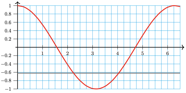
Figure \(\PageIndex{32}\)
Example \(\PageIndex{8}\) showcases the issue with using a graph to solve any equation—you get very rough approximations. In truth, the solutions to \( \cos(t) = -0.62 \) on the interval \( \left[ 0,2\pi \right] \) are approximately \( 2.2395 \) and \( 4.0436 \) (rounded to four decimal places). There is virtually no way to gain this level of accuracy using a hand-drawn graph.
An interesting observation comes from the fact that the sine and cosine curves oscillate forever in both directions. Had we not restricted our answers in Example \(\PageIndex{8}\) to lie between \( 0 \) and \( 2\pi \), we would have encountered an infinite number of times where the cosine curve intersects the line \( y = -0.62 \). Thus, the equation \( \cos(t) = -0.62 \) has an infinite number of solutions when considering all real numbers instead of restricting ourselves to the interval \( \left[ 0,2\pi \right] \).
Use a graph to find the two angles between \(0\) and \(2\pi\) that satisfy \(\sin (t) = -0.85\).
- Answer
-
Approximately \(4.14\) and \(5.25\)
This page titled 8.1: Base Graphs of the Fundamental Trigonometric Functions was last modified on Tue, 08 Jul 2025 17:45:09 GMT and is shared under a CC BY-SA 12 license and was authored, remixed, and/or curated by Roy Simpson.
The book could not be loaded just now.