Opening the book…
3.5 Relationship between Derivatives and the Shape of a Graph
- Use the first derivative of a function to determine the intervals where the function is increasing or decreasing, based on the sign of the derivative.
- Apply the first derivative test at critical points to determine whether a function has local extreme values (maximum or minimum) and identify their locations.
- Use the second derivative of a function to determine the intervals where the function is concave up or concave down, based on the sign of the second derivative.
- Apply the second derivative test at critical points to determine whether the function has local extrema and classify them as maxima, minima, or points of inflection.
Increasing–Decreasing Test:
- If \( f'(x) > 0 \) on an interval, then \( f \) is increasing on that interval.
- If \( f'(x) < 0 \) on an interval, then \( f \) is decreasing on that interval.
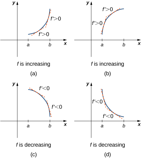
Figure \(\PageIndex{7}\): Functions describing when a function is decreasing or increasing. From OpenStax Calculus Volume 1, licensed under CC-BY-NC-SA.
The First Derivative Test:
Let \( f \) be a continuous function on an interval \( I \) containing a critical point \( c \) of \( f \). If \( f \) is differentiable on \( I \), except possibly at \( c \), then:
- If \( f' \) changes from positive to negative at \( c \), then \( f \) has a local maximum at \( c \). That is, \( f(c) \) is a local maximum value of \( f \).
- If \( f' \) changes from negative to positive at \( c \), then \( f \) has a local minimum at \( c \). That is, \( f(c) \) is a local minimum value of \( f \).
- If \( f' \) does not change sign at \( c \) (i.e., remains positive or negative on both sides), then \( f \) has no local maximum or minimum at \( c \).
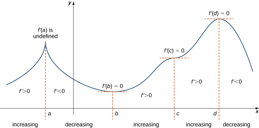
Figure \(\PageIndex{8}\): Several applications of the First Derivative Test to determine if the critical numbers of the function are local extrema. From OpenStax Calculus Volume 1, licensed under CC-BY-NC-SA.
Problem-Solving Strategy: Use the First Derivative Test to find local extreme values.
Suppose that \( f \) is continuous over an interval \( I \). Follow these steps to find local extrema:
- Find all critical points of \( f \), and divide the interval \( I \) into smaller subintervals using the critical points as endpoints.
- Analyze the sign of \( f' \) in each subinterval. Usually, \( f' \) is continuous over each subinterval, so its sign does not change within that subinterval. You can determine the sign of \( f' \) by choosing a test value \( x \) in the subinterval and evaluating \( f'(x) \).
- Use the sign of \( f' \) to determine whether \( f \) is increasing or decreasing over each subinterval.
- Apply the First Derivative Test using the results from Step 3 to determine whether \( f \) has a local maximum, a local minimum, or neither at each critical point.
Use the First Derivative Test to find the local extrema of the following functions, if any.
- \( y = x^3 - 6x^2 + 9x + 5 \)
- \( y = 2x^4 + 8x^3 + 9 \)
- \( y = 2(x^2 - 4)^3 \)
- \( y = 3x^2 e^x \)
- \( y = \dfrac{x^2 - 2x + 1}{x + 1} \)
Let \( f \) be a function that is differentiable over an open interval \( I \).
- If \( f' \) is increasing over \( I \), then \( f \) is said to be concave up on \( I \).
- If \( f' \) is decreasing over \( I \), then \( f \) is said to be concave down on \( I \).

Figure \(\PageIndex{9}\): Functions describing when a function is concave up or concave down. From OpenStax Calculus Volume 1, licensed under CC-BY-NC-SA.
Concavity Test:
- If \( f''(x) > 0 \) for all \( x \) in an interval \( I \), then the graph of \( f \) is concave up on \( I \).
- If \( f''(x) < 0 \) for all \( x \) in an interval \( I \), then the graph of \( f \) is concave down on \( I \).
Let \( f \) be a function continuous at \( x = a \). If \( f \) changes concavity at \( a \), then the point \( (a, f(a)) \) on the graph of \( f \) is called an inflection point. This means that \( (a, f(a)) \) is an inflection point of \( f \) if \( f''(a) = 0 \) or \( f''(a) \) is undefined,
and the concavity of \( f \) changes at that point.
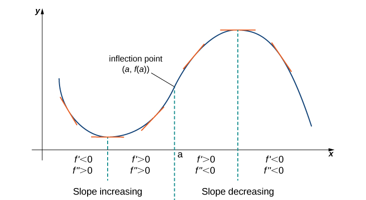
Figure \(\PageIndex{10}\): A function illustrating an inflection point. From OpenStax Calculus Volume 1, licensed under CC-BY-NC-SA.
For each of the following functions, determine:
- The intervals where the function is concave up.
- The intervals where the function is concave down.
- All inflection points of the function.
- \( y = x^4 - 4x^3 + 5 \)
- \(y= \frac{3}{20}x^5-\frac{3}{2}x^4+4x^3+3\)
- \( y =\dfrac{2x+8}{3x+3}\)
The Second Derivative Test:
Suppose that \( f'' \) is continuous near \( c \).
- If \( f'(c) = 0 \) and \( f''(c) > 0 \), then \( f \) has a local minimum at \( c \).
- If \( f'(c) = 0 \) and \( f''(c) < 0 \), then \( f \) has a local maximum at \( c \).
- If \( f'(c) = 0 \) and \( f''(c) = 0 \), then the test is inconclusive.

Figure \(\PageIndex{11}\): A function illustrating the Second Derivative Test. From OpenStax Calculus Volume 1, licensed under CC-BY-NC-SA.
Use the second derivative test to find the local extrema of the functions from Example 3.5.10.
This page titled 3.5: Relationship between Derivatives and the Shape of a Graph was last modified on Sun, 22 Mar 2026 18:00:38 GMT and is shared under a CC BY 4.0 license and was authored, remixed, and/or curated by Kevin Palencia.
The book could not be loaded just now.