Opening the book…
- Plot a curve described by parametric equations.
- Convert the parametric equations of a curve into the form \(y=f(x)\).
- Recognize the parametric equations of basic curves, such as a line and a circle.
In this section we examine parametric equations and their graphs. In the two-dimensional coordinate system, parametric equations are useful for describing curves that are not necessarily functions. The parameter is an independent variable that both \(x\) and \(y\) depend on, and as the parameter increases, the values of \(x\) and \(y\) trace out a path along a plane curve. For example, if the parameter is \(t\) (a common choice), then \(t\) might represent time. Then \(x\) and \(y\) are defined as functions of time, and \(\left(x(t),y(t)\right)\) can describe the position in the plane of a given object as it moves along a curved path.
Parametric Equations and Their Graphs
Consider the orbit of Earth around the Sun. Our year lasts approximately 365.25 days, but for this discussion we will use 365 days. On January 1 of each year, the physical location of Earth with respect to the Sun is nearly the same, except for leap years, when the lag introduced by the extra \(\dfrac{1}{4}\) day of orbiting time is built into the calendar. We call January 1 “day 1” of the year. Then, for example, day 31 is January 31, day 59 is February 28, and so on.
The number of the day in a year can be considered a variable that determines Earth’s position in its orbit. As Earth revolves around the Sun, its physical location changes relative to the Sun. After one full year, we are back where we started, and a new year begins. According to Kepler’s laws of planetary motion, the shape of the orbit is elliptical, with the Sun at one focus of the ellipse. We study this idea in more detail in Conic Sections.
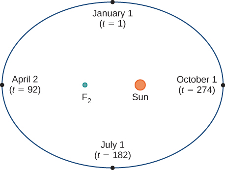
Figure \( \PageIndex{1}\) depicts Earth’s orbit around the Sun during one year. The point labeled \(F_2\) is one of the foci of the ellipse; the other focus is occupied by the Sun. If we superimpose coordinate axes over this graph, then we can assign ordered pairs to each point on the ellipse (Figure \( \PageIndex{2}\)). Then each \(x\) value on the graph is a value of position as a function of time, and each \(y\) value is also a value of position as a function of time. Therefore, each point on the graph corresponds to a value of Earth’s position as a function of time.
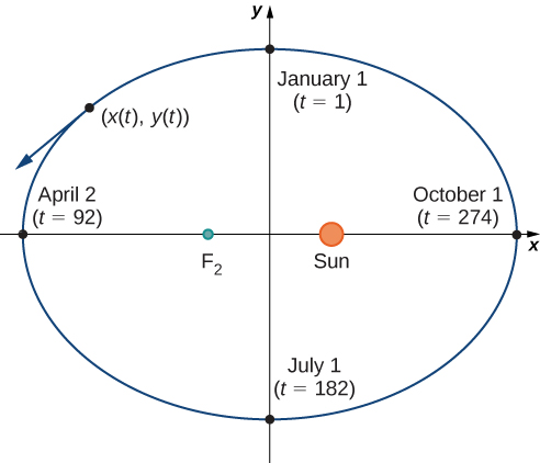
We can determine the functions for \(x(t)\) and \(y(t)\), thereby parameterizing the orbit of Earth around the Sun. The variable \(t\) is called an independent parameter and, in this context, represents time relative to the beginning of each year.
A curve in the \((x,y)\) plane can be represented parametrically. The equations that are used to define the curve are called parametric equations.
If \(x\) and \(y\) are continuous functions of \(t\) on an interval \(I\), then the equations
\[x=x(t) \quad \text{ and }\quad y=y(t) \nonumber \]
are called parametric equations and \(t\) is called the parameter. The set of points \((x,y)\) obtained as \(t\) varies over the interval \(I\) is called the graph of the parametric equations. The graph of parametric equations is called a parametric curve or plane curve, and is denoted by \(C\).
Notice in this definition that \(x\) and \(y\) are used in two ways. The first is as functions of the independent variable \(t\). As \(t\) varies over the interval \(I\), the functions \(x(t)\) and \(y(t)\) generate a set of ordered pairs \((x,y)\). This set of ordered pairs generates the graph of the parametric equations. In this second usage, to designate the ordered pairs, \(x\) and \(y\) are variables. It is important to distinguish the variables \(x\) and \(y\) from the functions \(x(t)\) and \(y(t)\).
Sketch the curves described by the following parametric equations:
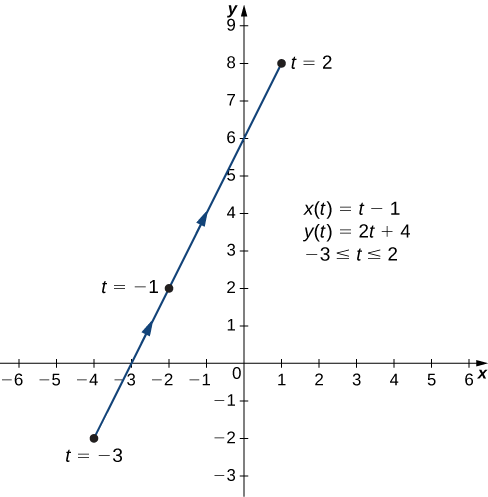
(a) \(\left\{\begin{array} {l} x(t) =t-1 \\ y(t) =2t+4 \end{array} \right. \quad \text{ for } −3≤t≤2\)
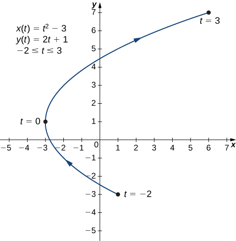
(b) \(\left\{\begin{array} {l} x(t) =t^2−3 \\ y(t) =2t+1 \end{array} \right. \quad \text{ for }−2≤t≤3\)
(c) \(\left\{\begin{array} {l} x(t) =4\cos(t) \\ y(t) =4\sin(t) \end{array} \right. \quad \text{ for }0≤t≤2π\)
Solution a
To create a graph of this curve, first set up a table of values. Since the independent variable in both \(x(t)\) and \(y(t)\) is \(t\), let \(t\) appear in the first column. Then \(x(t)\) and \(y(t)\) will appear in the second and third columns of the table.
| \(t\) | \(x(t)\) | \(y(t)\) |
|---|---|---|
| −3 | −4 | −2 |
| −2 | −3 | 0 |
| −1 | −2 | 2 |
| 0 | −1 | 4 |
| 1 | 0 | 6 |
| 2 | 1 | 8 |
The second and third columns in this table provide a set of points to be plotted. The graph of these points appears in Figure \( \PageIndex{3}\). The arrows on the graph indicate the orientation of the graph, that is, the direction that a point moves on the graph as t varies from −3 to 2.
Solution b
To create a graph of this curve, again set up a table of values.
| \(t\) | \(x(t)\) | \(y(t)\) |
|---|---|---|
| −2 | 1 | −3 |
| −1 | −2 | −1 |
| 0 | −3 | 1 |
| 1 | −2 | 3 |
| 2 | 1 | 5 |
| 3 | 6 | 7 |
The second and third columns in this table give a set of points to be plotted (Figure \( \PageIndex{4}\)). The first point on the graph (corresponding to \(t=−2\)) has coordinates \((1,−3)\), and the last point (corresponding to \(t=3\)) has coordinates \((6,7)\). As \(t\) progresses from \(−2\) to \(3\), the point on the curve travels along a parabola. The direction the point moves is again called the orientation and is indicated on the graph.
Solution c
In this case, use multiples of \(\dfrac{\pi}{6}\) for \(t\) and create another table of values:
| \(t\) | \(x(t)\) | \(y(t)\) | \(t\) | \(x(t)\) | \(y(t)\) |
|---|---|---|---|---|---|
| 0 | 4 | 0 | \(\dfrac{7π}{6}\) | \(-2\sqrt{3}≈−3.5\) | -2 |
| \(\dfrac{π}{6}\) | \(2\sqrt{3}≈3.5\) | 2 | \(\dfrac{4π}{3}\) | −2 | \(−2\sqrt{3}≈−3.5\) |
| \(\dfrac{π}{3}\) | 2 | \(2\sqrt{3}≈3.5\) | \(\dfrac{3π}{2}\) | 0 | −4 |
| \(\dfrac{π}{2}\) | 0 | 4 | \(\dfrac{5π}{3}\) | 2 | \(−2\sqrt{3}≈−3.5\) |
| \(\dfrac{2π}{3}\) | −2 | \(2\sqrt{3}≈3.5\) | \(\dfrac{11π}{6}\) | \(2\sqrt{3}≈3.5\) | -2 |
| \(\dfrac{5π}{6}\) | \(−2\sqrt{3}≈−3.5\) | 2 | \(2π\) | 4 | 0 |
| \(π\) | −4 | 0 |
The graph of this plane curve appears in the following graph.
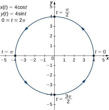
This is the graph of a circle with radius \(4\) centered at the origin, with a counterclockwise orientation. The starting point and ending points of the curve both have coordinates \((4,0)\).
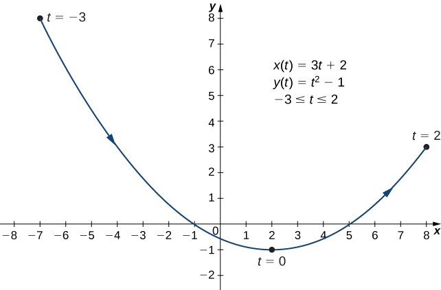
Sketch the curve described by the parametric equations
\[\left\{\begin{array} {l} x(t) =3t+2 \\ y(t) =t^2-1 \end{array} \right. \quad \text{ for }−3≤t≤2 \nonumber \]
- Hint
-
Make a table of values for \(x(t)\) and \(y(t)\) using \(t\) values from \(−3\) to \(2\).
- Answer
-
Eliminating the Parameter
To better understand the graph of a curve represented parametrically, it is useful to rewrite the two equations as a single equation relating the variables \(x\) and \(y\). Then we can apply any previous knowledge of equations of curves in the plane to identify the curve. For example, the equations describing the plane curve in Example \(\PageIndex{1b}\) are
\[\left\{\begin{array} {l} x(t) =t^2−3 \\ y(t) =2t+1 \end{array} \right. \quad \text{ for }-2\le t\le 3 \nonumber \]
Solving the second equation for \(t\) gives \(t=\dfrac{y-1}{2}\). This can be substituted into the top equation:
\[\begin{align*} x &=\left(\dfrac{y−1}{2}\right)^2−3 \\[4pt] x&=\dfrac{y^2−2y+1}{4}−3 \\[4pt] x&=\dfrac{y^2−2y−11}{4} \end{align*} \]
This equation describes \(x\) as a function of \(y\). These steps give an example of eliminating the parameter. The graph of this function is a parabola opening to the right (Figure \(\PageIndex{4}\)). Recall that the plane curve started at \((1,−3)\) and ended at \((6,7)\). These terminations were due to the restriction on the parameter \(t\).
Eliminate the parameter for each of the plane curves described by the following parametric equations and describe the resulting graph.
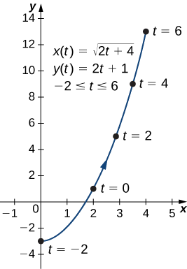
(a) \(\left\{\begin{array} {l} x(t) =\sqrt{2t+4} \\ y(t) =2t+1 \end{array} \right. \quad \text{ for }−2≤t≤6\)
(b) \(\left\{\begin{array} {l} x(t) =4\cos(t) \\ y(t) =3\sin(t) \end{array} \right. \quad \text{ for } 0≤t≤2π\)
Solution a
To eliminate the parameter, we can solve either of the equations for \(t\). For example, solving the first equation for \(t\) gives
\[\begin{align*} x &=\sqrt{2t+4} \\[4pt] x^2 &=2t+4 \\[4pt] x^2−4 &=2t \\[4pt] t &=\dfrac{x^2−4}{2} \end{align*}\]
Note that when we square both sides it is important to observe that \(x≥0\). Substituting \(t=\dfrac{x^2−4}{2}\) into \(y(t)\) yields
\[\begin{align*} y(t) &=2t+1 \\[4pt] y&=2\left(\dfrac{x^2−4}{2}\right)+1 \\[4pt] y&=x^2−4+1 \\[4pt] &\boxed{y=x^2−3} \nonumber \end{align*}\]
This is the equation of a parabola opening upward. There is, however, a domain restriction because of the limits on the parameter \(t\). When \(t=−2\), \(x=\sqrt{2(−2)+4}=0\), and when \(t=6\), \(x=\sqrt{2(6)+4}=4\). The graph of this plane curve follows.
Solution b
Sometimes it is necessary to be a bit creative in eliminating the parameter. The parametric equations for this example are
\[ x(t)=4 \cos (t)\nonumber \]
and
\[ y(t)=3 \sin (t)\nonumber \]
Solving either equation for \(t\) directly is not advisable because sine and cosine are not one-to-one functions. However, dividing the first equation by \(4\) and the second equation by \(3\) (and suppressing the \(t\)) gives us
\[ \cos (t)=\dfrac{x}{4}\quad \text{ and } \quad \sin (t)=\dfrac{y}{3} \nonumber \]
Now use the Pythagorean identity \(\cos^2(t)+\sin^2(t)=1\) and replace the expressions for \(\sin (t)\) and \(\cos(t)\) with the equivalent expressions in terms of \(x\) and \(y\):
\[ \left(\dfrac{x}{4}\right)^2+\left(\dfrac{y}{3}\right)^2=1 \nonumber \]
\[ \boxed{\dfrac{x^2}{16}+\dfrac{y^2}{9}=1} \nonumber \]
This is the equation of a horizontal ellipse centered at the origin, with semi-major axis \(4\) and semi-minor axis \(3\) as shown in the following graph.
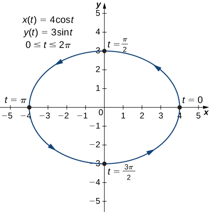
As \(t\) progresses from \(0\) to \(2π\), a point on the curve traverses the ellipse once, in a counterclockwise direction. Recall from the section opener that the orbit of Earth around the Sun is also elliptical. This is a perfect example of using parameterized curves to model a real-world phenomenon.
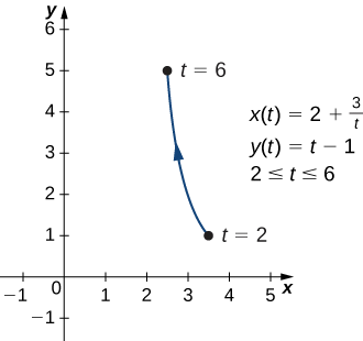
Eliminate the parameter for the plane curve defined by the following parametric equations and describe the resulting graph.
\[ \left\{\begin{array} {l} x(t) =2+\dfrac{3}{t} \\ y(t) =t-1 \end{array} \right. \quad \text{ for } 2≤t≤6 \nonumber \]
- Hint
-
Solve one of the equations for \(t\) and substitute into the other equation.
- Answer
-
\(x=2+\dfrac{3}{y+1},\) or \(y=−1+\dfrac{3}{x−2}\)
This equation describes a portion of a rectangular hyperbola centered at \((2,−1)\)
So far we have seen the method of eliminating the parameter, assuming we know a set of parametric equations that describe a plane curve. What if we would like to start with the equation of a curve and determine a pair of parametric equations for that curve? This is certainly possible, and in fact it is possible to do so in many different ways for a given curve. The process is known as parameterization of a curve.
We can find multiple different pairs of parametric equations to represent the graph of \(y=2x^2−3\)
First, it is always possible to parameterize a curve by defining \(x(t)=t\), then replacing \(x\) with \(t\) in the equation for \(y(t)\). This gives the parameterization
\[ \left\{\begin{array} {l} x(t) =t \\ y(t) =2t^2-3 \end{array} \right. \quad \text{ for } -\infty<t<\infty \nonumber \]
Since there is no restriction on the domain in the original graph, there is no restriction on the values of \(t\).
We have complete freedom in the choice for the second parameterization. For example, we can choose \(x(t)=3t−2\). The only thing we need to check is that there are no restrictions imposed on \(x\); that is, the range of \(x(t)\) is all real numbers. This is the case for \(x(t)=3t−2\). Now since \(y=2x^2−3\), we can substitute \(x(t)=3t−2\) for \(x\). This gives
\[ y(t)=2(3t−2)^2−2=2(9t^2−12t+4)−2=18t^2−24t+8−2=18t^2−24t+6 \nonumber \]
Therefore, a second parameterization of the curve can be written as
\( \left\{\begin{array} {l} x(t) =3t-2 \\ y(t) =18t^2-24t+6 \end{array} \right. \quad \text{ for } -\infty<t<\infty \)
Find two different sets of parametric equations to represent the graph of \(y=x^2+2x\)
- Hint
-
Follow the steps in Example \(\PageIndex{3}\). Remember we have freedom in choosing the parameterization for \(x(t)\).
- Answer
-
One possibility is \(\left\{\begin{array} {l} x(t) =t \\ y(t) =t^2+2t \end{array} \right. \)
Another possibility is \(\left\{\begin{array} {l} x(t) =2t-3 \\ y(t) =(2t-3)^2+2(2t-3) \end{array} \right. \quad \)
(There are, in fact, an infinite number of possibilities.)
Key Concepts
- Parametric equations provide a convenient way to describe a curve. A parameter can represent time or some other meaningful quantity.
- It is often possible to eliminate the parameter in a parameterized curve to obtain a function or relation describing that curve.
- There is always more than one way to parameterize a curve.
- Parametric equations can describe complicated curves that are difficult or perhaps impossible to describe using rectangular coordinates.
Glossary
- orientation
- the direction that a point moves on a graph as the parameter increases
- parameter
- an independent variable that both \(x\) and \(y\) depend on in a parametric curve; usually represented by the variable \(t\)
- parametric curve
- the graph of the parametric equations \(x(t)\) and \(y(t)\) over an interval \(a≤t≤b\) combined with the equations
- parametric equations
- the equations \(x=x(t)\) and \(y=y(t)\) that define a parametric curve
- parameterization of a curve
- rewriting the equation of a curve defined by a function \(y=f(x)\) as parametric equations
This page titled 10.1: Curves Defined by Parametric Equations was last modified on Tue, 14 Apr 2026 02:54:27 GMT and is shared under a CC BY-NC 4.0 license and was authored, remixed, and/or curated by Gilbert Strang & Edwin “Jed” Herman (OpenStax) via source content that was edited to the style and standards of the LibreTexts platform.
The book could not be loaded just now.