Opening the book…
- Substitute and multiply by monomials into known power series to represent similar functions.
- Differentiate and integrate known power series term-by-term to represent similar functions.
Representing Functions as Power Series
Being able to represent a function by an “infinite polynomial” is a powerful tool. Polynomial functions are the easiest functions to analyze, since they only involve the basic arithmetic operations of addition, subtraction, multiplication, and division. If we can represent a complicated function by an infinite polynomial, we can use the polynomial representation to differentiate or integrate it. In addition, we can use a truncated version of the polynomial expression to approximate values of the function. So, the question is, when can we represent a function by a power series?
Consider again the geometric series
\[1+x+x^2+x^3+\ldots =\sum_{n=0}^∞x^n \nonumber \]
Recall that the geometric series
\[a+ar+ar^2+ar^3+\ldots \nonumber \]
converges if and only if \(|r|<1.\) In that case, it converges to \(\dfrac{a}{1−r}\). Therefore, if \(|x|<1\), the series in Example \(\PageIndex{1}\) converges to \(\dfrac{1}{1−x}\) and we write
\[1+x+x^2+x^3+\ldots =\dfrac{1}{1−x} \text{ for }|x|<1 \nonumber \]
As a result, we are able to represent the function \(f(x)=\dfrac{1}{1−x}\) by the power series
\[1+x+x^2+x^3+\ldots \text{ when }|x|<1 \nonumber \]
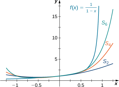
We now show graphically how this series provides a representation for the function \(f(x)=\dfrac{1}{1−x}\) by comparing the graph of \(f\) with the graphs of several of the partial sums of this infinite series.
Below, we sketched a graph of \(f(x)=\dfrac{1}{1−x}\) and the graphs of the corresponding partial sums \( \displaystyle S_N(x)=\sum_{n=0}^Nx^n\) for \(N=2,4,6\) on the interval \((−1,1)\).
From the graph in Figure \(\PageIndex{2}\), you see that as \(N\) increases, \(S_N\) becomes a better approximation for \(f(x)=\dfrac{1}{1−x}\) for \(x\) in the interval \((−1,1)\).
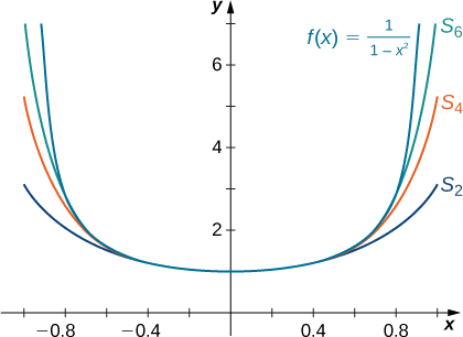
Sketch a graph of \(f(x)=\dfrac{1}{1−x^2}\) and the corresponding partial sums \(\displaystyle S_N(x)=\sum_{n=0}^Nx^{2n}\) for \(N=2,4,6\) on the interval \((−1,1).\)
- Hint
- \(S_N(x)=1+x^2+\ldots +x^{2N}=\dfrac{1−x^{2(N+1)}}{1−x^2}\)
- Answer
-
Next we consider functions involving an expression similar to the sum of a geometric series and show how to represent these functions using power series.
Use a power series to represent each of the following functions \(f\). Find the interval of convergence.
(a) \(f(x)=\dfrac{1}{1+x^3}\)
(b) \(f(x)=\dfrac{x^2}{4−x^2}\)
Solution
(a) You should recognize this function \(f\) as the sum of a geometric series, because
\[ \dfrac{1}{1+x^3}=\dfrac{1}{1−(−x^3)} \nonumber \]
Using the fact that, for \(|r|<1,\dfrac{a}{1−r}\) is the sum of the geometric series
\[ \sum_{n=0}^∞ar^n=a+ar+ar^2+\ldots \nonumber \]
we see that, for \(|−x^3|<1\):
\[ \begin{align*} \dfrac{1}{1+x^3} &=\dfrac{1}{1−(−x^3)} \\[4pt] &=\sum_{n=0}^∞(−x^3)^n \\[4pt] &=1−x^3+x^6−x^9+\ldots \end{align*}\]
Since this series converges if and only if \(|−x^3|<1\), the interval of convergence is \((−1,1)\), and we have
\[ \dfrac{1}{1+x^3}=1−x^3+x^6−x^9+\ldots \text{ for }|x|<1\nonumber \]
(b) This function is not in the exact form of a sum of a geometric series. However, with a little algebraic manipulation, we can relate f to a geometric series. By factoring 4 out of the two terms in the denominator, we obtain
\[ \begin{align*} \dfrac{x^2}{4−x^2} &=\dfrac{x^2}{4\left(\dfrac{1−x^2}{4}\right)}\\[4pt] &=\dfrac{x^2}{4\left(1−\left(\dfrac{x}{2}\right)^2\right)}\end{align*}\]
Therefore, we have
\[ \begin{align*} \dfrac{x^2}{4−x^2} &=\dfrac{x^2}{4\left(1−\left(\dfrac{x}{2}\right)^2\right)} \\[4pt]
&= \dfrac{\dfrac{x^2}{4}}{1−\left(\dfrac{x}{2}\right)^2} \\[4pt]
&= \sum_{n=0}^∞\dfrac{x^2}{4}\left(\dfrac{x}{2}\right)^{2n} \end{align*}\]
The series converges as long as \(\left|\left(\dfrac{x}{2}\right)^2\right|<1\) (note that when \(\left|\left(\dfrac{x}{2}\right)^2\right|=1\) the series does not converge). Solving this inequality, we conclude that the interval of convergence is \((−2,2)\) and
\[ \boxed{ \dfrac{x^2}{4−x^2} =\sum_{n=0}^∞\dfrac{x^{2n+2}}{4^{n+1}}} \text{ for } -2<x<2 \nonumber\]
Represent the function \(f(x)=\dfrac{x^3}{2−x}\) using a power series and find the interval of convergence.
- Hint
-
Rewrite f in the form \(f(x)=\dfrac{g(x)}{1−h(x)}\) for some functions \(g\) and \(h\).
- Answer
-
\(\displaystyle \sum_{n=0}^∞\dfrac{x^{n+3}}{2^{n+1}}\) with interval of convergence \((−2,2)\)
Term‑by‑Term Differentiation and Integration of Power Series
The real power of representing a function by a power series lies in how easily we can differentiate or integrate the series. For a polynomial, we differentiate or integrate term by term. The same is true for power series inside their interval of convergence.
Suppose the power series \(\displaystyle \sum_{n=0}^{\infty} c_n (x - a)^n\) has radius of convergence \(R > 0\) (or \(R = \infty\)). Then for \(|x - a| < R\):
- Term‑by‑term differentiation
\[ \frac{d}{dx} \left( \sum_{n=0}^{\infty} c_n (x - a)^n \right) = \sum_{n=1}^{\infty} n c_n (x - a)^{n-1} \nonumber \]
The new series has the same radius of convergence \(R\). - Term‑by‑term integration
\[ \int \left( \sum_{n=0}^{\infty} c_n (x - a)^n \right) dx = C + \sum_{n=0}^{\infty} c_n \frac{(x - a)^{n+1}}{n+1} \nonumber \]
The new series also has the same radius of convergence \(R\).
This means we can differentiate or integrate a known power series representation to obtain new power series for related functions without recomputing coefficients from scratch. For example, we know
\[ \frac{1}{1-x} = \sum_{n=0}^{\infty} x^n \quad \text{for } |x|<1 \nonumber \]
Differentiate both sides term-by-term:
\[ \frac{d}{dx} \left( \frac{1}{1-x} \right) = \frac{1}{(1-x)^2} \nonumber \]
\[ \frac{d}{dx} \left( \sum_{n=0}^{\infty} x^n \right) = \sum_{n=0}^{\infty} \frac{d}{dx} \left( x^{n} \right)= \sum_{n=0}^{\infty} n x^{n-1} \nonumber \]
Thus, we know that these quantities are equivalent:
\[ \frac{1}{(1-x)^2} = \sum_{n=0}^{\infty} nx^{n-1} \quad \text{for } |x|<1 \nonumber \]
The series on the right doesn't look precisely like a power series. It is worth noting that the first term (when \(n=0\)) is \(0x^{-1}=0\), so we can start the sum at \(n=1\) without losing any terms. Now we can do substitution on the index, letting \(m=n-1\). Just like in an integral, this changes the variables from \(n-1\) into \(m\), and the limits of the sum from \(n=1\) to \(m=0\) and from \(n=\infty\) to \(m=\infty\).
\[ \sum_{n=0}^{\infty} n x^{n-1} = \sum_{n=1}^{\infty} n x^{n-1} = \sum_{m=0}^{\infty} (m+1) x^{m} \nonumber \]
Therefore, we have found a new power series relationship:
\[ \frac{1}{(1-x)^2} = \sum_{n=0}^{\infty} (n+1) x^n \quad \text{for } |x|<1 \nonumber \]
Similarly, we can integrate both sides of our power series representation for \(\dfrac{1}{1-x}\) term-by-term:
\[ \int_0^x \frac{1}{1-t}\,dt = -\ln\left|1-t\right|\bigg|_0^x =-\ln|1-x| \nonumber \]
\[ \int_0^x \left( \sum_{n=0}^{\infty} t^n \right)\,dt = \sum_{n=0}^{\infty} \int t^n\,dt =\sum_{n=0}^\infty \dfrac{1}{n+1}t^{n+1}\bigg|_0^x = \sum_{n=0}^\infty \dfrac{x^{n+1}}{n+1} \nonumber \]
After another re-indexing substitution and multiplying both sides by \(-1\), we see that:
\[ \ln(1-x) = -\sum_{n=1}^{\infty} \frac{x^n}{n}\quad \text{for } |x|<1 \nonumber \]
Use a power series to represent each of the following functions \(f\). Find the interval of convergence.
(a) \(f(x)=\dfrac{1}{(1+2x)^2}\)
(b) \(f(x)=\dfrac{2x^2}{(1-x)^3}\)
(c) \(f(x)=\arctan(x)\)
Solution
(a) We begin with the geometric series \(\displaystyle \frac{1}{1-u} = \sum_{n=0}^{\infty} u^n\) for \(|u|<1\).
We have already shown that \(\dfrac{1}{(1-u)^2}\) is the derivative of this geometric series:
\[ \frac{d}{du}\left(\frac{1}{1-u}\right) = \frac{1}{(1-u)^2} = \sum_{n=1}^{\infty} n u^{n-1} = \sum_{n=0}^{\infty} (n+1) u^n \nonumber \]
Now we substitute \(u = -2x\)L
\[ \frac{1}{(1+2x)^2} =\dfrac{1}{\left(1-(-2x)\right)^2}= \sum_{n=0}^{\infty} (n+1) (-2x)^n = \sum_{n=0}^{\infty} (n+1)(-1)^n 2^n x^n \nonumber \]
The series converges when \(|u| = |{-2x}| < 1\), which is equivalent to \(|x| < \dfrac{1}{2}\). Checking the endpoints, we see that both diverge.
Thus, the interval of convergence is \(\left(-\dfrac{1}{2}, \dfrac{1}{2}\right)\), and
\[ \boxed{\frac{1}{(1+2x)^2} = \sum_{n=0}^{\infty} (n+1)(-1)^n 2^n x^n \quad \text{ for } |x|<\frac{1}{2}} \nonumber \]
(b) From part (a) with \(u\) replaced by \(x\), we have \(\displaystyle \frac{1}{(1-x)^2} = \sum_{n=0}^{\infty} (n+1) x^n\) for \(|x|<1\)
Differentiating and then re-indexing again gives us:
\[ \frac{d}{dx}\left(\frac{1}{(1-x)^2}\right) = \frac{2}{(1-x)^3} = \sum_{n=1}^{\infty} (n+1)n x^{n-1} = \sum_{n=0}^{\infty} (n+2)(n+1) x^n \nonumber \]
Therefore,
\[ \frac{2}{(1-x)^3} = \sum_{n=0}^{\infty} (n+2)(n+1) x^n \nonumber \]
Multiplying by \(x^2\) gives
\[ \frac{2x^2}{(1-x)^3} = x^2\cdot \sum_{n=0}^{\infty} (n+2)(n+1) x^{n}=\sum_{n=0}^{\infty} (n+2)(n+1) x^{n+2} \nonumber \]
Now we re-index with \(m=n+2\) to get:
\[ \sum_{n=0}^{\infty} (n+2)(n+1) x^{n+2}= \sum_{m=2}^{\infty} m(m-1) x^{m} \nonumber \]
Therefore, our final power series representation of \(f(x)\) is:
\[ \boxed{\frac{x^2}{(1-x)^3} = \sum_{n=2}^{\infty} n(n-1)x^n \quad \text{ for } |x|<1} \nonumber \]
(c) Recall that \(\displaystyle \frac{d}{dx} \big( \arctan (x)\big) = \frac{1}{1+x^2}\). We know the geometric series \(\displaystyle \frac{1}{1-u} = \sum_{n=0}^{\infty} u^n\) for \(|u|<1\). Let \(u = -x^2\):
\[ \frac{1}{1+x^2}=\dfrac{1}{1-\left(-x^2\right)} = \sum_{n=0}^{\infty} \left(-x^2\right)^n= \sum_{n=0}^{\infty} (-1)^n x^{2n} \quad \text{for } |x|<1 \nonumber \]
Integrate term by term from \(0\) to \(x\):
\[ \arctan(x)=\int_0^x \frac{1}{1+t^2} \,dt = \int_0^x \left( \sum_{n=0}^{\infty} (-1)^n t^{2n} \right) \,dt = \sum_{n=0}^{\infty} (-1)^n \int_0^x t^{2n} \,dt =\sum_{n=0}^{\infty} (-1)^n \frac{x^{2n+1}}{2n+1} \nonumber \]
The radius of convergence remains \(1\). At \(x = \pm 1\), the series becomes \(\displaystyle \sum (-1)^n \frac{(\pm 1)^{2n+1}}{2n+1}\), which converges by the Alternating Series Test. Thus the interval of convergence is \([-1, 1]\).
Therefore, we have shown that:
\[ \boxed{\arctan (x) = \sum_{n=0}^{\infty} (-1)^n \frac{x^{2n+1}}{2n+1} \quad \text{ for } -1 \le x \le 1} \nonumber \]
You might be tempted to think: “If we can add, subtract, differentiate, and integrate term‑by‑term, surely we can multiply two power series term‑by‑term as well?”
This is false — you cannot simply multiply corresponding terms.
For example, suppose
\[ A(x) = \sum_{n=0}^{\infty} a_n x^n, \quad B(x) = \sum_{n=0}^{\infty} b_n x^n \nonumber \]
The product \(A(x) \cdot B(x)\) is not \(\displaystyle \sum_{n=0}^{\infty} a_n b_n x^n\)
Example of the mistake:
Let \(A(x) = \dfrac{1}{1-x} = 1 + x + x^2 + \dots\) and \(B(x) = \dfrac{1}{1-x}\) (same function). Then \(A(x)B(x) = \dfrac{1}{(1-x)^2}\)
If we naively multiplied term‑by‑term:
\[ \left(1 + x + x^2 + \dots\right)\left(1 + x + x^2 + \dots\right) \text{ would be } 1 + x^2 + x^4 + \dots \nonumber \]
Notice that the resulting series would be \(\displaystyle \frac{1}{1-x^2}=\sum_{n=0}^\infty \left(x^2\right)^n \), which is not \(\dfrac{1}{(1-x)^2}\)
Indeed, we have already shown that \(\displaystyle \dfrac{1}{(1-x)^2} = \sum_{n=0}^\infty (n+1)x^n \), very different from \(\displaystyle \sum_{n=0}^\infty \left(x^2\right)^n \)
If you must multiply two power series, the correct product formula is know as the Cauchy product:
\[ A(x)B(x) = \sum_{n=0}^{\infty} \left( \sum_{k=0}^{n} a_k b_{n-k} \right) x^n \nonumber \]
Mixing up the two leads to serious errors.
Thus: Differentiate and integrate freely, but when multiplying power series, do not multiply term-by-term.
Use term‑by‑term differentiation of the geometric series to find a power series representation for \(\dfrac{2}{(2-x)^2}\)
- Answer
-
\(\displaystyle \frac{2}{(2-x)^2} = \sum_{n=0}^{\infty} \dfrac{n+1}{2^{n+1}} x^n\) for \(|x|<2\)
In the remaining sections of this chapter, we will show ways of deriving power series representations for many other functions, and how we can make use of these representations to evaluate, differentiate, and integrate various functions.
Key Concepts
- The geometric series \(\displaystyle \sum_{n=0}^∞x^n=\dfrac{1}{1−x}\) for \(|x|<1\) allows us to represent certain functions using geometric series.
- Inside its interval of convergence, a power series can be differentiated and integrated term‑by‑term, and the resulting series has the same radius of convergence.
- Differentiation and integration of known power series (like the geometric series) provide easy ways to obtain new series representations for related functions.
Key Equations
- Geometric Power Series center at \(x=0\)
\[ \sum_{n=0}^∞x^n=\dfrac{1}{1-x} \text{ when } -1<x<1 \nonumber \]
- Term‑by‑term differentiation (center at \(x=a\))
\[ \frac{d}{dx} \left( \sum_{n=0}^{\infty} c_n (x-a)^n \right) = \sum_{n=1}^{\infty} n c_n (x-a)^{n-1} \nonumber \]
- Term‑by‑term integration (center at \(x=a\))
\[ \int_a^x \left( \sum_{n=0}^{\infty} c_n (t-a)^n \right)\, dt = \sum_{n=0}^{\infty} c_n \frac{(x-a)^{n+1}}{n+1} \nonumber \]
This page titled 11.9: Representation of Functions as a Power Series was last modified on Tue, 14 Apr 2026 13:55:32 GMT and is shared under a CC BY-NC 4.0 license and was authored, remixed, and/or curated by Gilbert Strang & Edwin “Jed” Herman (OpenStax) via source content that was edited to the style and standards of the LibreTexts platform.
The book could not be loaded just now.