Opening the book…
- Apply a formula to model the exponential relationship between two variables.
- Apply the natural growth formula to solve the problem.
- Apply the logistic growth formula to solve the problem.
Exponential Growth
Suppose that every year, only \(10\%\) of the fish in a lake have surviving offspring. Assuming that none of the adult fish dies, if there were \(100\) fish in the lake last year, there would now be \(110\) fish. If there were \(1000\) fish in the lake last year, there would now be \(1100\) fish. Absent any inhibiting factors, populations of people and animals tend to grow by a percentage of the existing population each year. Whenever a quantity grows by a fixed percentage rather than a fixed amount, the growth is exponential, like compound interest.
Suppose our lake began with \(1000\) fish, and \(10\%\) of the fish have surviving offspring each year. Since we start with \(1000\) fish, \(P_0 = 1000\). How do we calculate \(P_1\)? The new population will be the old population plus an additional \(10\%\). Symbolically:
\[P_1=P_0+0.10P_0\nonumber\]
Notice this could be condensed to a shorter form by factoring:
\[P_{1}= P_{0}+0.10 P_{0}=(1+0.10) P_{0}=1.10 P_{0}\nonumber\]
While \(10\%\) is the growth rate, \(1.10\) is the growth multiplier. Notice that \(1.10\) can be thought of as “the original \(100\%\) plus an additional \(10\%\)”, which is \(110\%\) (of the original population).
For our fish population,
\[P_{0}=1.10(1000)=1100\nonumber\]
We could then calculate the population in later years:
\[P_{2}=1.10 P_{1}=1.10(1100)=1210\nonumber\]
\[P_{3}=1.10 P_{2}=1.10(1210)=1331\nonumber\]
Notice that in the first year, the population grew by \(100\) fish; in the second year, the population grew by \(110\) fish; and in the third year, the population grew by \(121\) fish. While there is a constant percentage growth, the actual increase in number of fish is increasing each year.

Graphing these values reveals that this growth doesn’t appear to be linear.
To gain a clearer understanding of how this percentage-based growth impacts things, we need an explicit formula to quickly calculate values further into the future.
Like we did for the linear model, we will start building from the recursive equation:
\[\begin{array}{l}
P_{1}=1.10 P_{0}=1.10(1000) \\
P_{2}=1.10 P_{1}=1.10(1.10(1000))=1.10^{2}(1000) \\
P_{3}=1.10 P_{2}=1.10\left(1.10^{2}(1000)\right)=1.00^{3}(1000) \\
P_{4}=1.10 P_{3}=1.10\left(1.10^{3}(1000)\right)=1.10^{4}(1000)
\end{array} \nonumber \]
Observing a pattern, we can generalize the explicit form to be:
\(P_{n}=1.10^{n}(1000)\) or equivalently, \(P_{n}=1000\left(1.10^{n}\right)\). This is exactly like the compound interest formula with \(r=10 \% \) annually.
From this, we can quickly calculate the number of fish in \(10, 20,\) or \(30\) years:
\[\begin{array}{l}
P_{10}=1.10^{10}(1000)=2594 \\
P_{20}=1.10^{20}(1000)=6727 \\
P_{30}=1.10^{30}(1000)=17,449
\end{array} \nonumber \]
Adding these values to our graph reveals a shape that is definitely not linear. If our fish population had been growing linearly, by \(100\) fish each year, the population would have only reached \(4000\) in \(30\) years, compared to almost \(18,000\) with this percent-based growth, called exponential growth.
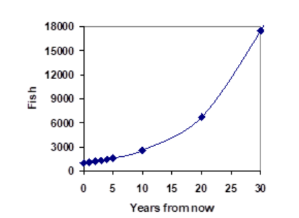
In exponential growth, the population grows proportionally to its own size, so as the population increases, the same percentage growth will yield a larger numeric growth.
If a quantity starts at size \(P_0\) and grows (or decays) by \(r\% \) (written as a decimal) every time period, then the quantity after \(n\) time periods can be determined by following the model (function).
| Exponential Growth | Exponential Decay |
|---|---|
| \[P(n)=P_{0}(1+r)^n\nonumber\] | \[P(n)=P_{0}(1-r)^n\nonumber\] |
Where \(P(n)=P_{n}\), which is the population (or amount) after \(n\) time.
\(P(0)=P_{0}\), which is the population (or amount) in the beginning or the initial amount.
We call \(r\) the growth (decay) rate. Usually, it is expressed as a percentage, but you need to convert it to a decimal when you put it into the equation.
The term \((1+r)\) is called the growth (decay) multiplier, or growth (decay) factor, or common ratio.
Formula for Growth Factor if \(P(0)\) and \(P(1)\) are given
\begin{align*}
\text{Growth Factor}&=\frac{P_{1}}{P_{0}}\\
\end{align*}
If we know the growth factor, we can find the growth rate using the following formula
\begin{align*}
\text{Growth Rate}&=\text{Growth Factor}-1\\
\end{align*}
Additionally, we can express the explicit form slightly differently, as shown below, with \(n\) time periods denoted as \(t\).
\[f(t)=ab^{t}\nonumber\]
Where \(f(t)\) is similar to \(P(t)\), \(P(0)\) similar to \(a\), and \(1+r\) is similar to \(b\). The two formulas above can be combined into a single formula in word.
\[
\boxed{\text{Amount after time \(t\)}=\text{Initial Amount}\times(\text{Growth Factor})^{t}\nonumber
}
\]
If growth factor \(b\) is \(>1\), the model \(f(x)\) is called an exponential growth model.
If growth factor \(b\) is \(<1\), the model \(f(x)\) is called an exponential decay model.
A friend is using the equation \(P_n=4600(1.072)^n\) to predict the annual tuition at a local college. She says the formula is based on years after \(2010\). What does this equation tell us?
In the equation, \(P_0 = 4600\) is the tuition's starting value when \(n = 0\). This tells us that the tuition in \(2010\) was \($4,600.\)
The growth multiplier or growth factor is \(1.072\).
\begin{align*}
\text{Growth Rate}&=\text{Growth Factor}-1\\
&=1.072-1\\
&=0.072\\
&=7.2\%
\end{align*}
This tells us that the tuition is expected to grow by \(7.2\%\) yearly.
Putting this together, we could say that the tuition in \(2010\) was \($4,600\) and is expected to grow by \(7.2\%\) each year.
Example \(\PageIndex{2}\): Use Exponential Model Function
Between \(2007\) and \(2008,\) Olympia, WA, grew by almost \(3\%\) to a population of \(245\) thousand people. If this growth rate were to continue, what would the population of Olympia be in \(2014?\)
- Answer
-
As we did before, we first need to define which year corresponds to \(n = 0\). Since we know the population in \(2008,\) it would make sense to have \(2008\) correspond to \(n = 0\), so \(P_0 = 245,000.\)The year \(2014\) would then be \(2014-2008 = 6.\)
We know the growth rate is \(3\%,\) giving \(r = 0.03\).
Using the model function:
\begin{align*}
P(6)=P_{6}&=245,000(1+0.03)^{6}\\
&=245,000\times1.19405\\
&=292,542.25
\end{align*}The model predicts that in \(2014,\) Olympia would have a population of about \(293\) thousand people.
Here's a simple table showing exponential growth over time.
| Time, \(t\) | \(0\) | \(1\) | \(2\) | \(3\) | \(4\) | \(5\) | \(6\) | \(7\) | \(8\) | \(9\) | \(10\) |
|---|---|---|---|---|---|---|---|---|---|---|---|
| Value, \(P(t)\) | \(100\) | \(150\) | \(225\) | \(337.5\) | \(506.25\) | \(759.38\) | \(1139.06\) | \(1708.59\) | \(2562.89\) | \(3844.34\) | \(5766.51\) |
What is an exponential model equation representing the above table?
Here, \(P_0 = 100\), \(P_1 = 150\), \(P_2 = 225\) and so on.
Since the growth factor is a common ratio. To find it, we have to divide the one value by the value that follows it.
\[\text{Growth factor }= \frac{P_1}{P_0} = \frac{150}{100}=1.5\nonumber\] and
\begin{align*}\text{Growth Rate}&=\text{Growth Factor}-1\\
&=1.50 -1\\
&=0.50\\
&=50\%
\end{align*}
So, the exponential model is
\[P_{t} = P_{0}(1+r)^{t}=100(1.5)^t\nonumber\]
The graph of the above model is shown below.

Figure \(\PageIndex{3}\): Exponential Growth, Growth rate \(50\%\)
What is the predicted value when \( t= 25.\) To find it, we put in the model equation
\[P_{25}=P_{0}(1+r)^{t}=100(1.5)^{25}=2,525,116.829\nonumber\]
Example \(\PageIndex{4}\) : Find Exponential Model

The table above shows a person's bank account balance for \(5\) years.
- Find the growth factor and growth rate.
- Find an exponential model for this data, with \(y\) representing the balance \(t\) years after \(1998\) and \(t=0\) corresponding to \(1998\).
- Find this person's balance in \(2010\) if the bank account continues to grow at the same rate.
- Answer
-
- Here, \(P_0 = 8000\), \(P_1 = 8440\), \(P_2 = 8904.20\) and so on.\begin{align*}\text{Growth Factor:~}(1+r)&=\frac{P_1}{P_0}\\&=\frac{8440}{8000}\\&=1.055\\\end{align*} In the above exponential model, the growth rate is \( 5.5\%\). See the calculation below\begin{align*}\text{Growth Rate}&=\text{Growth Factor}-1\\&=1.055-1\\&=0.055\\&=5.5\%\end{align*}
- The exponential model in is\[y=P_{t}=P(t)=P_{0}(1+r)^{t}=8000(1.055)^t\nonumber\]
- To find the predicted balance in \(2010,\) which is \( t= 2010-1998=12\) years after \(1998,\) we put \(t=12\) into the equation
\begin{align*}
P(t)&=P_{0}(1+r)^{t}\\
P(12)&=8000(1.055)^{12}\\
&=15209.65989\\
\end{align*}So this person's balance in \(2010\) will be \($15209.66.\) Round to two decimal places.
Your Turn \( \PageIndex{4} \): Use Exponential Formula
Example \(\PageIndex{5}\) : Use Exponential Model
A population grows according to an exponential growth model. The initial population is \(P_{0} = 19\), and the growth rate is \(r = 15\%\).
- Find the exponential model that predicts the population after \(n\) period.
- Find \(P_{1}\) and \(P_{2}\).
- Find \(P_{10}\).
- Answer
-
-
The exponential model is
\[P_{n}=19(1+0.15)^{n}=19(1.15)^n\nonumber\]
-
To find \(P(1)\), put \(n=1\) in the model
\begin{align*}P(1)&=P_{0}(1+r)^n\\
&=19(1.15)^1\\
&=21.85\end{align*}
To find \(P(2)\), put \(n=2\) in the model
\begin{align*}
P(1)&=P_{0}(1+r)^n\\
&=19(1.15)^2\\
&=25.1275
\end{align*} - To find \(P_{10}\). we put \(n=10\) into above model
\begin{align*}
P_{10}&=19\times(1.15)^{10}\\
&=76.87\\
\end{align*}
-
Natural Growth
In this section, we will examine natural and logistic growth. Most naturally occurring phenomena grow continuously. That is called natural growth. Population growth is usually modeled using natural growth models, which are also exponential. However, they use the mathematical constant e as the base. The growth rate per given period, k, is a part of the exponent, which is multiplied by the number of periods.
Natural growth is a form of exponential growth involving the mathematical constant e, approximately equal to ≈ 2.718.
The Natural Growth Model is
\[P(t)=P_{0} e^{k t} \nonumber \]
where \(P_{0}\) is the initial population, \(k\) is the growth rate per unit of time, and \(t\) is the number of time periods.
Note: \(P(t)\) is same as \(P_t\).
The Natural Decay Model is
\[P(t)=P_{0} e^{-k t} \nonumber \]
where \(P_{0}\) is the initial population, \(k\) is the decay rate per unit of time, and \(t\) is the number of time periods.
Note: \(P(t)\) is same as \(P_t\).


Example \(\PageIndex{6}\): Natural Decay
When a certain drug is administered to a patient, the number of milligrams remaining in the bloodstream after t hours is given by the model
\[P(t) = 40e^{-0.25t} \nonumber \]
How many milligrams are in the blood after two hours?
- Answer
-
To solve this problem, we use the given equation with \(t=2\). Here growth rate is \(0.25,\) which is same as \(25\%.\)
\begin{aligned}
P(2) &= 40e^{-0.25(2)} \\
&= 24.26
\end{aligned}There are approximately \(24.6\) milligrams of the drug in the patient’s bloodstream after two hours.
Example \(\PageIndex{7}\): Natural Growth
Bob has an ant problem. On the first day of May, Bob discovers he has a small red ant hill in his backyard, with a population of about \(100\) ants. If conditions are just right, red ant colonies will have a growth rate of \(240\%\) per year during the first four years. If Bob does nothing, how many ants will he have next May? How many in five years?
- Answer
-
We solve this problem using the natural growth model. Here \(k=2.40.\)
\[P(t) = 100e^{2.4t} \nonumber \]
In one year, \( t = 1\), we have
\[P(1) = 100e^{2.4(1)} = 1102 \text{ ants} \nonumber \]
In one year, \( t = 5\), we have
\[P(5) = 100e^{2.4(5)} = 16,275,479 \text{ ants} \nonumber \]
That is a lot of ants! Bob will not let this happen in his backyard!
Figure \(\PageIndex{3}:\) Graph of Ant Population Growth in Bob’s Yard. Note: The population of ants in Bob’s backyard follows an exponential (or natural) growth model.
The problem with exponential growth is that the population grows without bound, and at some point, the model will no longer predict what is actually happening because the amount of resources available is limited. Populations cannot continue to grow on a purely physical level; eventually, death occurs, and a limiting population is reached.
Logistic Growth Model
Another growth model for living organisms is the logistic growth model. In the real world, "unlimited" doesn't last. Space runs out, food becomes scarce, and waste builds up. This introduces the concept of Carrying Capacity \(C\), the maximum population an environment can sustain. The logistic growth model has a maximum population, known as the carrying capacity. As the population grows, it reaches the carrying capacity and remains there. This is the maximum population the environment can sustain. Logistic growth is used to model situations where growth starts out exponentially but then slows down as it approaches a maximum limit (called the carrying capacity).
For our fish, the carrying capacity is the largest population that the resources in the lake can sustain. If the population in the lake is far below the carrying capacity, then we would expect the population to grow essentially exponentially. However, as the population approaches the carrying capacity, there will be a scarcity of food and space available, and the growth rate will decrease. If the population exceeds the carrying capacity, there won’t be enough resources to sustain all the fish and there will be a negative growth rate, causing the population to decrease back to the carrying capacity.
The carrying capacity, or maximum sustainable population, is the largest population that an environment can support.
\[P_t=P(t) = \dfrac{C}{1+\left(\frac{C}{P_0}-1\right)e^{-rt}} \nonumber \]
where \(P(t)\) = Population over the time \(t\)
\(C\) = Carrying capacity
\(r\) = growth rate
\(t\) = time
\(P(0) = P_0\) = Initial Population
Note: \(P(t)\) is same as \(P_t\).


Figure \(\PageIndex{4}\): Logistic (Right) and Exponential (Left) Model Graph
The horizontal line on this graph illustrates the carrying capacity.
(Logistic Growth Image 1, n.d.)
(Logistic Growth Image 2, n.d.)
The graph for logistic growth starts with a small population. When the population is small, the growth is fast because there is more elbow room in the environment. As the population approaches the carrying capacity, the growth slows.
Example \(\PageIndex{8}\): Bird Population
The population of an endangered bird species on an island grows according to the logistic growth model.
\[P(t) = \dfrac{3640}{1+25e^{-0.04t}} \nonumber \]
Identify the initial population. What will the bird population be in five years? What will the population be like in \(150\) years? What will the population be like in \(500\) years?
- Answer
-
We know the initial population, \(P_{0}\), occurs when \(t = 0.\)
\[P_{0} = P(0) = \dfrac{3640}{1+25e^{-0.04(0)}} = \dfrac{3640}{1+25\times1} =140 \nonumber \]
Note: \(e^{-0.04(0)}=e^0=1\)
When \(t = 5\), calculate the population in five years.
\[P(5) = \dfrac{3640}{1+25e^{-0.04(5)}} = 169.6 \nonumber \]
The island will be home to approximately \(170\) birds in five years
Calculate the population in \(150\) years, when \(t = 150\).
\[P(150) = \dfrac{3640}{1+25e^{-0.04(150)}} = 3427.6 \nonumber \]
The island will be home to approximately \(3428\) birds in \(150\) years.
Calculate the population in \(500\) years when \(t = 500\).
\[P(500) = \dfrac{3640}{1+25e^{-0.04(500)}} = 3640.0 \nonumber \]
The island will be home to approximately \(3640\) birds in \(500\) years.
This example shows that the population grows quickly between five years and \(150\) years, with an overall increase of over \(3000\) birds, but slows dramatically between \(150\) years and \(500\) years (a longer span of time) with an increase of just over \(200\) birds.
Figure \(\PageIndex{6}:\) Bird Population over a \(200\)-Year Span
Example \(\PageIndex{9}\): Logistic Model
Suppose \(16\) blackberry plants started growing in a yard. Absent constraint, the number of blackberry plants will increase continuously at a monthly rate of \(80\%.\) If the yard can only sustain \(150\) plants, use a logistic growth model to estimate the number of plants after \(4\) months.
- Answer
-
The following formula gives the logistic growth model. \[P(t) = \dfrac{C}{1+\left(\frac{C}{P_0}-1\right)e^{-rt}} \nonumber \] Where
\(C= 150\)
\(P_0=16\)
\(r= 80\% = 0.8\)
Put those values in the given model.
\begin{align*}
P(t) &= \dfrac{C}{1+\left(\frac{C}{P_0}-1\right)e^{-rt}}\\
P(4) &= \dfrac{150}{1+\left(\frac{150}{16}-1\right)e^{-0.80t}} \\
&= \dfrac{150}{1+8.375e^{-0.80\times 4}}\\
&=111.82484
\end{align*}
After \(4\) month, there will be about \(112\) blackberry plants.
This page titled 2.2: Exponential, Natural, and Logistic Models was last modified on Mon, 13 Apr 2026 23:55:16 GMT and is shared under a CC BY license and was authored, remixed, and/or curated by Cheban Acharya.
The book could not be loaded just now.