Opening the book…
- Determine whether an ordered pair is a solution to a linear inequality in two variables
- Sketch the set of all solutions to a linear inequality in two variables, including correct shading and boundary line
- Sketch the set of all solutions ot a system of linear inequalities, including correct shading and boundary lines
- Explain the similarities and differences between a linear inequality in one variable, a linear inequality in two variables, and a system of linear inequalities
- Use the notation and techniques of systems of linear inequalities to find solutions to real-world problems
Previously, we graphed inequalities in one variable, but now we learn to graph inequalities in two variables. Although this section may seem similar to linear equations in two variables, linear inequalities in two variables have many applications. For example, business owners want to know when revenue is greater than cost so that their business makes a profit, e.g., revenue \(>\) cost.
Verifying Solutions
An ordered pair \((x, y)\) is a solution to a linear inequality in two variables, \(ax + by < c\), if the ordered pair \((x, y)\) makes the inequality true, where the the same is for \(>,\: ≤,\: ≥\) and \(a,\: b\neq 0\).
Verify whether each ordered pair is a solution to the inequality \(y > x + 4\).
- \((0,0)\)
- \((1,6)\)
Solution
We substitute the ordered pairs into the inequality and determine if the results are true.
- Let’s substitute \((0, 0)\) into the inequality and determine if the left side is greater than the right side. \[\begin{array}{rl}y\stackrel{?}{>}x+4&\text{Substitute }x=0\text{ and }y=0 \\ 0\stackrel{?}{>}0+4&\text{Simplify} \\ 0\ngtr 4&\text{ False}\end{array}\nonumber\] Hence, \((0,0)\) is not a solution to the inequality \(y>x+4\).
- Let’s substitute \((1, 6)\) into the inequality and determine if the left side is greater than the right side. \[\begin{array}{rl}y\stackrel{?}{>}x+4&\text{Substitute }x=1\text{ and }y=6 \\ 6\stackrel{?}{>}1+4&\text{Simplify} \\ 6>5&\checkmark\text{ True}\end{array}\nonumber\] Hence, \((1,6)\) is a solution to the inequality \(y>x+4\).
Boundary Lines
If we are given a linear inequality, \(ax + by < c\), we can see that not all ordered pairs are a solution, only some. Why? Well, notice that \((0, 0)\) is below the line \(y = x + 4\) and \((1, 6)\) is above the line \(y = x + 4\). This implies that ordered pairs in certain regions are solutions to the inequality \(y > x + 4\). Hence, the line \(y = x + 4\) is critical when finding solutions to the inequality. We call the line \(y = x + 4\) a boundary line, a line that separates the ordered pairs that are solutions and the ordered pairs that are not solutions of the linear inequality in two variables \(y > x + 4\).
A linear equation in two variables \(ax + by = c\) is called the boundary line, the line that separates the region where \(ax + by > c\) from the region where \(ax + by < c\).
Since there are four inequality symbols: \(>,\: <,\: \geq ,\: \leq\), then we have linear inequalities in two variables that include the boundary, e.g., inequalities with \(\leq\) and \(\geq\), and linear inequalities in two variables that exclude the boundary, e.g., inequalities with \(<\) and \(>\).
We can use the table below to help identify the boundary line, determine whether to include it, and visualize its graphical representation.
| Case 1. | Case 2. |
|---|---|
| \(ax+by<c\) | \(ax+by\leq c\) |
| \(ax+by>c\) | \(ax+by\geq c\) |
| Boundary line: \(ax+by=c\) | Boundary line: \(ax+by=c\) |
| Boundary line is excluded in solution | Boundary line is included in solution |
| Boundary line is dashed | Boundary line is solid |
Let’s revisit the first example and graph the boundary line, as well as the points \((0, 0)\) and \((1, 6)\).
Solution
Since we have \(y > x + 4\), we can see from the table above that we have Case 1, and the boundary line is excluded. We represent this by graphing the line \(y = x + 4\) as a dashed line.

We can see from the graph that the point \((0, 0)\) lies below the boundary line \(y = x + 4\) and point \((1, 6)\) lies above the boundary line. Recall, point \((1, 6)\) was verified as a solution of \(y > x + 4\). Furthermore, any ordered pair that lies above \(y = x+ 4\) will verify as a solution, i.e., making the inequality true. We typically represent this area by shading the region where the set of ordered pairs satisfies the inequality.
Graphing Linear Inequalities
Given a linear inequality in two variables, \(ax + by < c\), we can use the steps below to graph \(ax + by < c\), where the the same process is applied for \(>,\: ≤,\: ≥\) and \(a,\: b\neq 0\).
Step 1. Rewrite the inequality in slope-intercept form, i.e., \(y = mx + b\).
Step 2. Graph the boundary line according to the two cases:
Case 1. If the inequality is \(<\) or \(>\), then the boundary line is dashed.
Case 2. If the inequality is \(≥\) or \(≤\), then the boundary line is solid.
Step 3. Select a test point that is not on the boundary line. Ask: Does this ordered pair make the inequality true?
Step 4. If the ordered pair is
- a solution to the inequality, i.e., makes the inequality true, then shade the side that includes the ordered pair.
- not a solution, then shade the opposite side of the boundary line.
If we choose a test point on the boundary line, we will obtain an identity, where both sides of the inequality symbol are the same number. Hence, it is crucial to select a point that is not on the boundary line.
Graph the inequality: \[2x − y > 3\nonumber .\]
Solution
Let’s follow the steps given above to graph the inequality.
Step 1. Rewrite the inequality in slope-intercept form, i.e., \(y = mx + b\). \[\begin{aligned} 2x-y&>3 \\ -y&>-2x+3 \\ y&<2x-3\end{aligned}\]
Step 2. Graph the boundary line according to the two cases. Since the given inequality is \(<\), then we have Case 1.

Step 3. Select a test point that is not on the boundary line. Ask: Does this ordered pair make the inequality true?
Let’s pick the test point \(\color{red}{(0, 0)}\) as it is a great choice! \[\begin{aligned} y&\stackrel{?}{<}2x-3 \\ 0&\stackrel{?}{<}2(0)-3 \\ 0&\nless -3\end{aligned}\] Hence, \((0,0)\) doesn't make the inequality true.
Step 4. If the ordered pair is
- a solution to the inequality, i.e., makes the inequality true, then shade the side that includes the ordered pair.
- not a solution, then shade the opposite side of the boundary line.
Since the ordered pair \((0, 0)\) is not a solution to the inequality, we shade on the opposite side of the boundary line from the location of the ordered pair.

Another way of graphing linear inequalities in two variables is to complete Step 1. and Step 2., but instead of taking a test point in Step 3., we can observe the inequality symbols. If the inequality has \(y<\) or \(y≤\), then we shade below the boundary line, i.e., below the \(y\)-intercept. Similarly, if the inequality has \(y>\) or \(y\geq\), then we shade above the boundary line, i.e., above the \(y\)-intercept.
Graph the inequality: \[3x + 2y ≥ −6.\nonumber\]
Solution
Let’s follow the steps given above to graph the inequality, but try skipping Step 3. and Step 4.
Step 1. Rewrite the inequality in slope-intercept form, i.e., \(y = mx + b\). \[\begin{aligned}3x+2y&\geq -6 \\ 2y&\geq -3x-6 \\ y&\geq -\frac{3}{2}x-3\end{aligned}\]
Step 2. Graph the boundary line according to the two cases. Since the given inequality is \(≥\), then the boundary line is solid.

Since this inequality is \(y\geq\), where all ordered pairs above the boundary line are solutions to the inequality, we can easily shade above the \(y\)-intercept:

Determine whether an ordered pair is a solution of a system of linear inequalities
The definition of a system of linear inequalities is similar to that of a system of linear equations.
Two or more linear inequalities grouped together form a system of linear inequalities.
A system of linear inequalities resembles a system of linear equations, but it contains inequalities instead of equations. A system of two linear inequalities is shown here.
\[\left\{\begin{array} {l} x+4y\geq 10\\3x−2y<12\end{array}\right.\nonumber\]
To solve a system of linear inequalities, we will find values of the variables that are solutions to both inequalities. We solve the system by using the graphs of each inequality and show the solution as a graph. We will find the region on the plane that contains all ordered pairs \((x,y)\) that make both inequalities true.
Solutions of a system of linear inequalities are the values of the variables that make all the inequalities true.
The solution of a system of linear inequalities is represented as a shaded region in the \(xy\)-coordinate system, encompassing all points whose ordered pairs satisfy the inequalities.
To determine if an ordered pair is a solution to a system of two inequalities, we substitute the values of the variables into each inequality. If the ordered pair satisfies both inequalities, it is a solution to the system.
Determine whether the ordered pair is a solution to the system \(\left\{\begin{array} {l} x+4y\geq 10\\3x−2y<12\end{array}\right.\)
a. \((−2,4)\) b. \((3,1)\)
Solution:
a. Is the ordered pair \((−2,4)\) a solution?
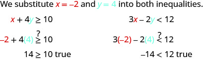
The ordered pair \((−2,4)\) made both inequalities true. Therefore \((−2,4)\) is a solution to this system.
b. Is the ordered pair \((3,1)\) a solution?
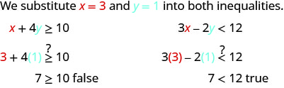
The ordered pair \((3,1)\) made one inequality true, but the other one false. Therefore \((3,1)\) is not a solution to this system.
Solve a System of Linear Inequalities by Graphing
The solution to a single linear inequality is the region on one side of the boundary line that contains all the points that make the inequality true. The solution to a system of two linear inequalities is a region that contains the solutions to both inequalities. To find this region, we will graph each inequality separately and then identify the region where both inequalities are true. The solution is always shown as a graph.
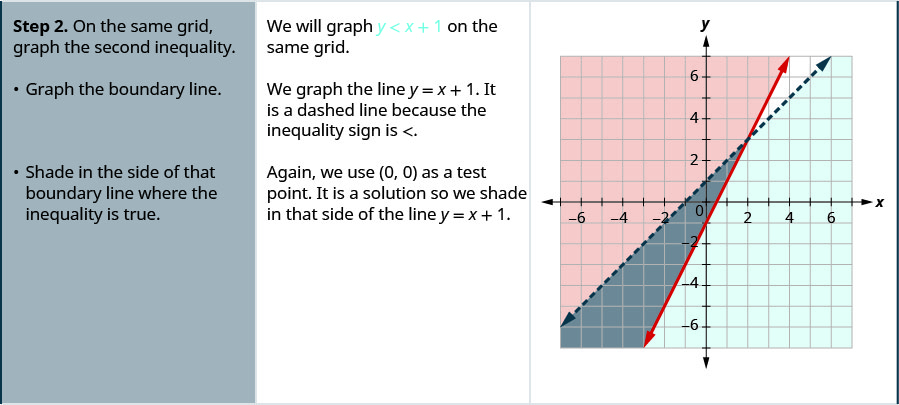
Solve the system by graphing: \(\left\{\begin{array} {l} y\geq 2x−1 \\ y<x+1\end{array}\right.\)
Solution:
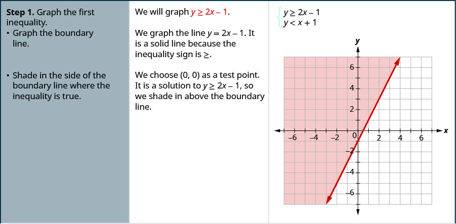

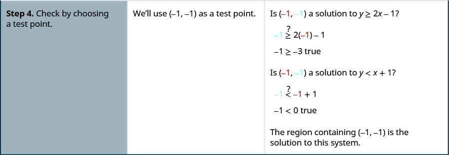
- Graph the first inequality.
- Graph the boundary line.
- Shade the side of the boundary line where the inequality is true.
- On the same grid, graph the second inequality.
- Graph the boundary line.
- Shade in the side of that boundary line where the inequality is true.
- The solution is the region where the shading overlaps.
- Check by choosing a test point.
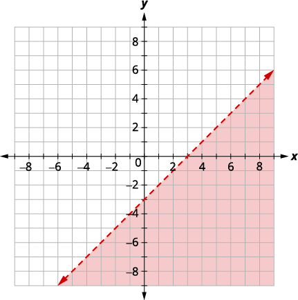
Solve the system by graphing: \(\left\{\begin{array} {l} x−y>3\\y<−\dfrac{1}{5}x+4\end{array}\right.\)
Solution:
| \(\left\{\begin{array} {l} x−y>3\\y<−\dfrac{1}{5}x+4\end{array}\right.\) | |
| Graph \(x - y > 3,\) by graphing \(x - y = 3\) and testing a point. The intercepts are \(x = 3\) and \(y = −3\) and the boundary line will be dashed. Test \((0, 0)\) which makes the inequality false so shade (red) the side that does not contain \((0, 0).\) |
 |
|
Graph \(y<−\dfrac{1}{5}x+4\) by graphing \(y=−\dfrac{1}{5}x+4\) |
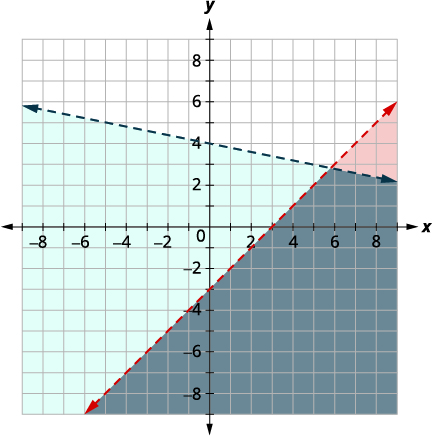 |
The point of intersection of the two lines is not included, as both boundary lines were dashed. The solution is the area shaded twice, which appears as the darkest shaded region.
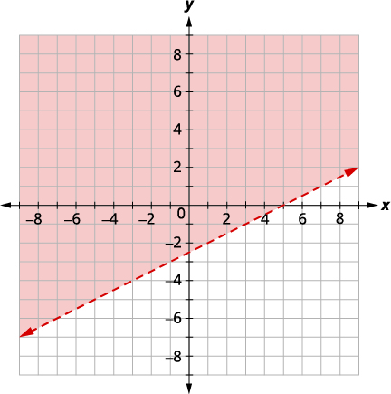
Solve the system by graphing: \(\left\{\begin{array} {l} x−2y<5\\y>−4\end{array}\right.\)
Solution:
| \(\left\{\begin{array} {l} x−2y<5\\y>−4\end{array}\right.\) | |
| Graph \(x−2y<5\), by graphing \(x−2y=5\) and testing a point. The intercepts are \(x = 5\) and \(y = −2.5\) and the boundary line will be dashed. Test \((0, 0)\) which makes the inequality true, so shade (red) the side that contains \((0, 0).\) |
 |
| Graph \(y>−4\), by graphing \(y=−4\) and recognizing that it is a horizontal line through \(y=−4\). The boundary line will be dashed. Test \((0, 0)\) which makes the inequality true so shade (blue) the side that contains \((0, 0).\) |
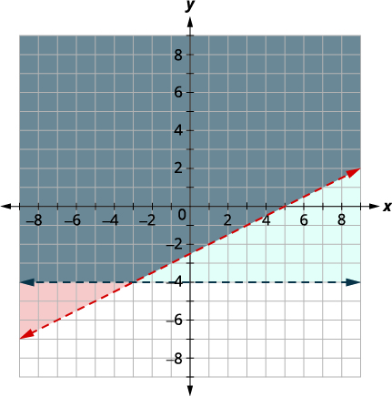 |
The point \((0,0)\) is in the solution, and we have already found it to be a solution of each inequality. The point of intersection of the two lines is not included, as both boundary lines were dashed.
The solution is the area shaded twice, which appears as the darkest shaded region.
Systems of linear inequalities where the boundary lines are parallel might have no solution. We’ll see this in the next example.
Solve the system by graphing: \(\left\{\begin{array} {l} 4x+3y\geq 12 \\ y<−\frac{4}{3}x+1\end{array}\right.\)
Solution:
| \(\left\{\begin{array} {l} 4x+3y\geq 12 \\ y<−\frac{4}{3}x+1\end{array}\right.\) | |
|
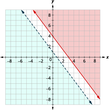 |
There is no point of intersection between the two shaded regions, so the system has no solution.
Some systems of linear inequalities with parallel boundary lines will have a solution. We’ll see this in the next example.
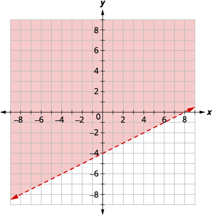
Solve the system by graphing: \(\left\{\begin{array} {l} y>\frac{1}{2}x−4\\x−2y<−4\end{array}\right.\)
Solution:
| \(\left\{\begin{array} {l} y>\frac{1}{2}x−4\\x−2y<−4\end{array}\right.\) | |
| Graph \(y>\frac{1}{2}x−4\) by graphing \(y=\frac{1}{2}x−4\) using the slope \(m=\frac{1}{2}\) and the intercept \(b = −4.\) The boundary line will be dashed. Test \((0, 0)\) which makes the inequality true, so shade (red) the side that contains \((0, 0).\) |
 |
| Graph \(x−2y<−4\) by graphing \(x−2y=−4\) and testing a point. The intercepts are \(x = -4\) and \(y=2\) and the boundary line will be dashed. Choose a test point in the solution and verify that it is a solution to both inequalties. Test \((0, 0)\) which makes the inequality false, so shade (blue) the side that does not contain \((0, 0).\) |
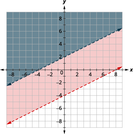 |
No point on the boundary lines is included in the solution as both lines are dashed.
The solution is the region that is shaded twice, which is also the solution to \(x−2y<−4\).
Solve Applications of Systems of Inequalities
To solve applications of systems of inequalities, we translate each condition into an inequality. Then, we graph the system, as we did above, to see the region that contains the solutions. Many situations will be realistic only if both variables are positive, so we add inequalities to the system as additional requirements.
Christy sells her photographs at a street fair. At the start of the day, she wants to have at least 25 photos to display at her booth. Each small photo she displays costs her $4, and each large photo costs her $10. She doesn’t want to spend more than $200 on photos to display.
a. Write a system of inequalities to model this situation.
b. Graph the system.
c. Could she display 10 small and 20 large photos?
d. Could she display 20 large and 10 small photos?
Solution:
a.
\(\begin{array} {ll} \text{Let} &{x=\text{the number of small photos.}} \\ {} &{y=\text{the number of large photos}}\end{array}\)
To find the system of equations translate the information.
\( \qquad \begin{array} {l} \\ \\ \text{She wants to have at least 25 photos.} \\ \text{The number of small plus the number of large should be at least }25. \\ \hspace{45mm} x+y\geq 25 \\ \\ \\ $4 \text{ for each small and }$10\text{ for each large must be no more than }$200 \\ \hspace{40mm} 4x+10y\leq 200 \\ \\ \\ \text{The number of small photos must be greater than or equal to }0. \\ \hspace{50mm} x\geq 0 \\ \\ \\ \text{The number of large photos must be greater than or equal to }0. \\ \hspace{50mm} y\geq 0 \end{array} \)
We have our system of equations.
\(\hspace{65mm} \left\{\begin{array} {l} x+y\geq 25 \\4x+10y\leq 200\\x\geq 0\\y\geq 0\end{array}\right.\)
b.
Since \(x\geq 0\) and \(y\geq 0\) (both are greater than or equal to) all solutions will be in the first quadrant. As a result, our graph shows only quadrant one.
| To graph \(x+y\geq 25\), graph \(x+y=25\) as a solid line. Choose \((0, 0)\) as a test point. Since it does not make the inequality true, shade (red) the side that does not include the point \((0, 0).\) To graph \(4x+10y\leq 200\), graph \(4x+10y=200\) as a solid line. Choose \((0, 0)\) as a test point. Since it does make the inequality true, shade (blue) the side that include the point \((0, 0).\) |
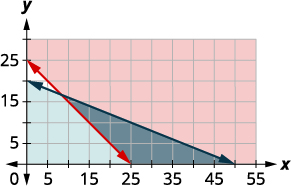 |
The solution of the system is the region of the graph that is shaded the darkest. The boundary line sections that border the darkly-shaded section are included in the solution, as are the points on the \(x\)-axis from \((25, 0)\) to \((55, 0).\)
c. To determine if 10 small and 20 large photos would work, we look at the graph to see if the point \((10, 20)\) is in the solution region. We could also test the point to see if it is a solution of both equations.
It is not, Christy would not display 10 small and 20 large photos.
d. To determine if 20 small and 10 large photos would work, we look at the graph to see if the point \((20, 10)\) is in the solution region. We could also test the point to see if it is a solution to both equations.
It is, so Christy could choose to display 20 small and 10 large photos.
Notice that we could also test the possible solutions by substituting the values into each inequality.
When we use variables other than \(x\) and \(y\) to define an unknown quantity, we must change the names of the axes of the graph as well.
Omar needs to eat at least 800 calories before going to his team practice. All he wants is hamburgers and cookies, and he doesn’t want to spend more than $5. At the convenience store near his college, each hamburger has 240 calories and costs $1.40. Each cookie has 160 calories and costs $0.50.
a. Write a system of inequalities to model this situation.
b. Graph the system.
c. Could he eat 4 cookies and 1 hamburger?
d. Could he eat 1 cookie and 4 hamburgers?
Solution:
a.
\(\begin{array} {ll} \text{Let} & c=\text{the number of cookies} \\ &h=\text{the number of hamburgers.}\end{array}\)
To find the system of equations, translate the information.
The calories from hamburgers at 240 calories each, plus the calories from cookies at 160 calories each must be more that 800.
\(\qquad \begin{array} {l} \hspace{40mm} 240h+160c\geq 800 \\ \\ \\ \text{The amount spent on hamburgers at }$1.40\text{ each, plus the amount spent on cookies}\\\text{at }$0.50\text{ each must be no more than }$5.00.\\ \hspace{40mm} 1.40h+0.50c\leq 5 \\ \\ \\ \text{The number of hamburgers must be greater than or equal to 0.} \\ \hspace{50mm} h\geq 0 \\ \text{The number of cookies must be greater than or equal to 0.}\\ \hspace{50mm} c\geq 0 \end{array} \)
\(\text{We have our system of equations.} \qquad \left\{ \begin{array} {l} 240h+160c\geq 800 \\ 1.40h+0.50c\leq 5 \\ h\geq 0 \\ c\geq 0\end{array} \right.\)
b.
Since \(h\geq 0\) and \(c\geq 0\) (both are greater than or equal to), all solutions will be in the first quadrant. As a result, our graph shows only quadrant one.
| To graph \(240h+160c\geq 800\), graph \(240h+160c=800\) as a solid line. Choose \((0, 0)\) as a test point. Since it does not make the inequality true, shade (red) the side that does not include the point \((0, 0).\) |
 |
Graph \(1.40h+0.50c\leq 5\). The boundary line is \(1.40h+0.50c=5\). We test \((0, 0)\) and it makes the inequality true. We shade the side of the line that includes \((0, 0).\)
The solution of the system is the region of the graph that is shaded the darkest. The boundary line sections that border the darkly shaded section are included in the solution as are the points on the \(x\)-axis from \((5, 0)\) to \((10, 0).\)
c. To determine if 4 cookies and 1 hamburger would meet Omar’s criteria, we see if the point \((4, 1)\) is in the solution region. It is, so Omar might choose this option.
d. To determine if 1 cookie and 4 hamburgers would meet Omar’s criteria, we see if the point \((1, 4)\) is in the solution region. It is not, so Omar should not choose this option.
We could also test the possible solutions by substituting the values into each inequality.
This page titled 1.5: Two Variable Linear Inequalities and Systems was last modified on Fri, 29 Aug 2025 03:30:38 GMT and is shared under a CC BY-NC 4.0 license and was authored, remixed, and/or curated by Math Department via source content that was edited to the style and standards of the LibreTexts platform.
The book could not be loaded just now.