1.2: Plotting in the Cartesian Plane

The Cartesian Plane (commonly called the \(xy\)-plane) has the following components:

While plotting points in quadrants may grow dull quickly, the Cartesian plane is a powerful tool. We can use this plane to help visualize relationships between the variables \(x\) and \(y\) by plotting a dot on every point which satisfies it. The resulting shape is a graph unique to the given relationship.

When the equation looks like \(Ax+By=C\), the graph looks like a straight line.
Any straight line can be drawn by finding any two points on that line.
To find these points, you can pick any value of \(x\) or \(y\) to plug in, and then solve for the other variable in the equation. If plugging in \(x=a\) gives an equation that has solution \(y=b\) (or if plugging in \(y=b\) gives an equation with solution \(x=a\)) then plot the point \((a,b)\).

Example \(\PageIndex{1}\)

Sketch the graph of \(\textcolor{brown}{2x+y=2}\)

Solution

We plug in a few different x values, and solve the equation they form for y:

Plug in	Equation Becomes	Solution
\(\textcolor{blue}{x=0}\)	\(2\cdot 0+y=2\)	\(\textcolor{blue}{y=2}\)
\( \textcolor{green!40!black!70}{x=1}\)	\(2\cdot 1+y=2\)	\( \textcolor{green!40!black!70}{y=0}\)
\(\textcolor{red}{x=2}\)	\(2\cdot 2+y=2\)	\(\textcolor{red}{y=-2}\)

Now we plot these points and connect any two of them to draw the graph of our line.

Example \(\PageIndex{2}\)

Sketch the graph of \(\textcolor{brown}{-x+3y=6}\)

Solution

This time we plug in a few different y values, and solve the equation they form for x:

Plug in	Equation Becomes	Solution
\(\textcolor{blue}{y=1}\)	\(-x+3\cdot 1 =6\)	\(\textcolor{blue}{x=-3}\)
\( \textcolor{green!40!black!70}{y=2}\)	\(-x+3\cdot 2 =6\)	\( \textcolor{green!40!black!70}{x=0}\)
\(\textcolor{red}{y=3}\)	\(-x+3\cdot 3 =6\)	\(\textcolor{red}{x=3}\)

Again we plot these points and connect any two of them to draw the graph of our line.

Example \(\PageIndex{3}\)

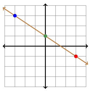
Sketch the graph of \(\textcolor{brown}{y=-\dfrac{2}{3}x+1}\)

Solution

We plug in a few friendly x values, and solve the equation they form for y:

Plug in	Equation Becomes	Solution
\(\textcolor{blue}{x=-3}\)	\(y=-\dfrac{2}{3}\cdot (-3)+1\)	\(\textcolor{blue}{y=3}\)
\( \textcolor{green!40!black!70}{x=0}\)	\(y=-\frac{2}{3}\cdot 0+1\)	\( \textcolor{green!40!black!70}{y=1}\)
\(\textcolor{red}{x=3}\)	\(y=-\frac{2}{3}\cdot 3+1\)	\(\textcolor{red}{y=-1}\)

Again we plot these points and connect any two of them to draw the graph of our line.

Example \(\PageIndex{4}\)

Sketch the graph of \(\textcolor{brown}{y+1=-3(x-2)}\)

Solution

We plug in a few friendly x values, and solve the equation they form for y:

Plug in	Equation Becomes	Solution
\(\textcolor{blue}{x=1}\)	\(y+1=-3(1-2)\)	\(\textcolor{blue}{y=2}\)
\( \textcolor{green!40!black!70}{x=2}\)	\(y+1=-3(2-2)\)	\( \textcolor{green!40!black!70}{y=-1}\)
\(\textcolor{red}{x=3}\)	\(y+1=-3(2-3)\)	\(\textcolor{red}{y=-4}\)

Again we plot these points and connect any two of them to draw the graph of our line.

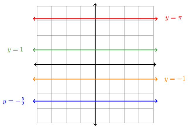
Of course in \(Ax+By=C\), if \(A\) or \(B\) are zero, then one of the variables disappears, giving either the line \(x=\alpha\) or \(y=\beta\).

For lines of the form \(y=\beta\), note that for any real number \(a\), if you plug in \(x=a\) the result is always \(y=\beta\). This means the point \((a,\beta)\) must be on this line for all values of \(a\). The resulting picture will contain all points which have the fixed \(y\)-value of \(\beta\), which gives a horizontal line.

For lines of the form \(x=\alpha\), note that for any real number \(b\), if you plug in \(y=b\) the result is always \(x=\alpha\). This means the point \((\alpha,b)\) must be on this line for all values of \(b\). The resulting picture will contain all points which have the fixed \(x\)-value of \(\alpha\), which gives a vertical line.

---