9.3: The Inverse Trigonometric Functions — Read

From LibreTexts, under CC BY-NC-SA 4.0, as the source states it; its equations are written in TeX, which the PDF shows typeset. This page at LibreTexts.

Remember that not all functions have an inverse. $y=f(x)$ needs to pass the horizontal line test on its domain in order for the function $f^{-1}(x)$ to exist. Sadly, every trigonometric function we have seen fails the horizontal line test spectacularly. Since these functions repeat every $2\pi$, we will need to restrict their domain appropriately if we want to make them invertible.

There are many different ways we could do this, but since we were born a few centuries too late to be the first people trying this, we will just go with what is considered the standard domain for each:

SINE

$f(x)=\sin(x)$ with domain $\textcolor{red}{\displaystyle{\left[ -\frac{\pi}{2},\frac{\pi}{2}\right]}}$

$clipboard_e29fb2a7ee0ecb7d48a56639e26fb8f36.png$

The red portion of this graph clearly passes the horizontal line test, so $f^{-1}$ should exist:

$f^{-1}(x)=\sin^{-1}(x)$

$clipboard_ec0742c7fdc6a78b86f36068a82937f05.png$

We can easily see the domain of $\sin^{-1}(x)$ is $[-1,1]$ and the range is $\displaystyle{\left[ -\frac{\pi}{2},\frac{\pi}{2}\right]}$

Remember inverses are supposed to compose with each other and "cancel out".
In other words, that means $\sin^{-1}(x)$ is the value of $\displaystyle{t\in \left[ -\frac{\pi}{2},\frac{\pi}{2}\right]}$ that makes $\sin(t)=x$

For example: $\textcolor{blue}{\displaystyle{\sin^{-1}\left( \frac{1}{2}\right)=\frac{\pi}{6}}}$ since $\textcolor{blue}{\displaystyle{\sin\left( \frac{\pi}{6}\right)=\frac{1}{2}}}$

Even though $\textcolor{purple}{\displaystyle{\sin\left( \frac{5\pi}{6}\right)=\frac{1}{2}}}$ , since $\displaystyle{\frac{5\pi}{6}}$ is not in the range of $\sin^{-1}(x)$, it is not the right answer! We need to be careful and pick the answer from the correct interval in order to be well defined.

COSINE

Since using $\displaystyle{\left[ -\frac{\pi}{2},\frac{\pi}{2}\right]}$ would not make cosine one-to-one, we use a different restricted domain:

$f(x)=\cos(x)$ with domain $\textcolor{red}{\left[ 0,\pi\right]}$

$clipboard_e1923f09495bfde340691494d11099eea.png$

Again the red portion of this graph passes the horizontal line test, so $f^{-1}$ should exist:

$f^{-1}(x)=\cos^{-1}(x)$

$clipboard_e61d44b894bc9bf12c4453524d690a599.png$

We can easily see the domain of $\cos^{-1}(x)$ is $[-1,1]$ and the range is $\left[ 0,\pi \right]$

Therefore this means that $\cos^{-1}(x)$ is the angle $t\in [0,\pi]$ that satisfies $\cos(t)=x$

For example: $\textcolor{blue}{\displaystyle{\cos^{-1}(0)=\frac{\pi}{2}}}$ since $\textcolor{blue}{\displaystyle{\cos\left( \frac{\pi}{2}\right)=0}}$

It is worth noting that for each of the last two graphs, since $\sin(x)$ and $\cos(x)$ were continuous on the restricted domains, their inverses were also continuous functions. This will always be the case: the inverse of a continuous function is continuous.

TANGENT

This time using $\displaystyle{\left[ -\frac{\pi}{2},\frac{\pi}{2}\right]}$ again does make tangent one-to-one, but $\displaystyle{x=-\frac{\pi}{2}}$ and $\displaystyle{x=\frac{\pi}{2}}$ are not technically in the domain of tangent at all, so we use $\displaystyle{\left( -\frac{\pi}{2},\frac{\pi}{2}\right)}$ :

$f(x)=\tan(x)$ with domain $\textcolor{red}{\displaystyle{\left(-\frac{\pi}{2},\frac{\pi}{2}\right)}}$

$clipboard_e8c290201bedb7357071b0c0ce6fa2492.png$

Once again the red portion of this graph passes the horizontal line test, so $f^{-1}$ should exist:

$f^{-1}(x)=\tan^{-1}(x)$

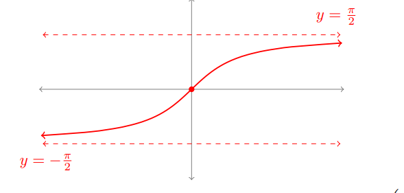
$clipboard_eb61b3d02652507eb5b52c303e773158f.png$

We can clearly see the domain of $\tan^{-1}(x)$ is $(-\infty,\infty)$ and the range is $\displaystyle{\left( -\frac{\pi}{2},\frac{\pi}{2} \right)}$

Again this means that $\tan^{-1}(x)$ is the angle $\displaystyle{t\in \left( -\frac{\pi}{2},\frac{\pi}{2} \right)}$ that satisfies $\tan(t)=x$

For example: $\textcolor{blue}{\displaystyle{\tan^{-1}\left(-\sqrt{3}\right)=-\frac{\pi}{3}}}$ since $\textcolor{blue}{\displaystyle{\tan\left( -\frac{\pi}{3}\right)=\frac{\sin\left(-\frac{\pi}{3}\right)}{\cos\left( -\frac{\pi}{3}\right)}=\frac{-\frac{\sqrt{3}}{2}}{\frac{1}{2}}=-\sqrt{3}}}$

It is a good idea to become familiar with the values of $\tan(t)$ for $t$ in this range:

$\displaystyle{\tan\left( -\frac{\pi}{3}\right)=-\sqrt{3}}$ $\displaystyle{\tan\left( \frac{\pi}{3}\right)=\sqrt{3}}$

$\displaystyle{\tan\left( -\frac{\pi}{4}\right)=-1}$ $\displaystyle{\tan\left( \frac{\pi}{4}\right)=1}$

$\displaystyle{\tan\left( -\frac{\pi}{6}\right)=-\frac{1}{\sqrt{3}}}$ $\displaystyle{\tan\left( \frac{\pi}{6}\right)=\frac{1}{\sqrt{3}}}$

and of course $\tan(0)=0$

COTANGENT

For cotangent to be one-to-one, we use $\left(0,\pi\right)$ as the restricted domain:

$f(x)=\cot(x)$ with domain $\textcolor{red}{\left( 0,\pi\right)}$

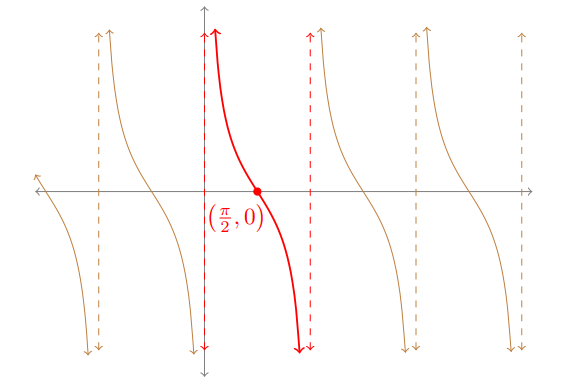
$clipboard_ee23b2bda1f9ebd31ffd56b007b0e6bf0.png$

Once more the red portion of this graph passes the horizontal line test, so $f^{-1}$ should exist:

$f^{-1}(x)=\cot^{-1}(x)$

$clipboard_e389bef6be824b7b4bceb347a2384c7ca.png$

We can see the domain of $\cot^{-1}(x)$ is $(-\infty,\infty)$ and the range is $\left( 0,\pi \right)$

Therefore this means that $\cot^{-1}(x)$ is the angle $t\in (0,\pi)$ that satisfies $\cot(t)=x$

For example: $\textcolor{blue}{\displaystyle{\cot^{-1}\left( -\frac{1}{\sqrt{3}}\right)=\frac{2\pi}{3}}}$ since $\textcolor{blue}{\displaystyle{ \cot\left( \frac{2\pi}{3}\right)=\frac{\cos\left( \frac{2\pi}{3}\right)}{\sin\left( \frac{2\pi}{3}\right)}=\frac{-\frac{1}{2}}{\frac{\sqrt{3}}{2}}=-\frac{1}{\sqrt{3}}}}$

It is also worth it to become familiar with the values of $\cot(t)$ for $t$ in this range:

$\displaystyle{\cot\left( \frac{\pi}{3}\right)=\sqrt{3}}$ $\displaystyle{\cot\left( \frac{2\pi}{3}\right)=-\sqrt{3}}$

$\displaystyle{\cot\left( \frac{\pi}{4}\right)=1}$ $\displaystyle{\cot\left( \frac{3\pi}{4}\right)=-1}$

$\displaystyle{\cot\left( \frac{\pi}{6}\right)=\frac{1}{\sqrt{3}}}$ $\displaystyle{\cot\left( \frac{5\pi}{6}\right)=-\frac{1}{\sqrt{3}}}$

and of course $\displaystyle{\cot\left(\frac{\pi}{2}\right)=0}$

SECANT

The last two trigonometric functions (secant and cosecant) are the most interesting.

It would be reasonable to pick $\textcolor{green}{\displaystyle{\left[0,\frac{\pi}{2}\right)\cup \left(\frac{\pi}{2},\pi\right]}}$ for secant, since these intervals make $\sec(x)$ one-to-one and closely align with the restrictions for cosine we used earlier

(with the vertical asymptote $\displaystyle{x=\frac{\pi}{2}}$ removed)

In fact, many books and online resources actually use this restriction.

But some books (like this one) choose a different domain: $\textcolor{red}{\displaystyle{\left[0,\frac{\pi}{2}\right) \cup \left[ \pi, \frac{3\pi}{2}\right)}}$

This makes a difference because these domains effect what the derivative of these graphs look like:

$y=\sec(x)$

$clipboard_e1f74db23b36c43575d6220dbd2540820.png$

In the green regions, $\sec(x)$ is always increasing, so its derivative will always be positive.
(This means its inverse will always have a positive derivative too since they are reciprocals!)

But for the red regions, $\sec(x)$ can be increasing or decreasing, so its derivative (and thus the derivative of its inverse) will have both positive and negative values.

When we solve for the derivatives of these inverses soon, it will be easier to deal with the red version. That is why this author chooses the restricted domain $\textcolor{red}{\displaystyle{\left[0,\frac{\pi}{2}\right) \cup \left[ \pi, \frac{3\pi}{2}\right)}}$ for $\sec(x)$.

This leads us to the graph of $y=\sec^{-1}(x)$:

$clipboard_edd01a183a67615002a262bfb031f9b53.png$

We can see the domain of $\sec^{-1}(x)$ is $(-\infty,-1]\cup[1,\infty)$ and the range is $\displaystyle{\left[ 0,\frac{\pi}{2}\right)\cup\left[\pi,\frac{3\pi}{2} \right)}$

Therefore this means that $\sec^{-1}(x)$ is the angle $\displaystyle{t\in\left[ 0,\frac{\pi}{2}\right)\cup\left[\pi,\frac{3\pi}{2} \right)}$ that satisfies $\sec(t)=x$

COSECANT

For the same reasons as we saw in secant, we will choose to restrict cosecant's domain to $\textcolor{red}{\displaystyle{\left(0,\frac{\pi}{2}\right] \cup \left(\pi,\frac{3\pi}{2}\right]}}$ instead of $\textcolor{green}{\displaystyle{\left[-\frac{\pi}{2},0\right)\cup \left( 0,\frac{\pi}{2}\right]}}$ (which some books choose to use)

$f(x)=\csc(x)$ with domain $\textcolor{red}{\displaystyle{\left(0,\frac{\pi}{2}\right] \cup \left(\pi,\frac{3\pi}{2}\right]}}$

$clipboard_e338e24b62deefbd2cc19f6cf8bb3f9e1.png$

This is clearly invertible and leads us to the graph of $y=\csc^{-1}(x)$:

$clipboard_e215cde6baf687caf95c7c93f2b3b5b03.png$

We can see the domain of $\csc^{-1}(x)$ is $(-\infty,-1]\cup[1,\infty)$ and the range is $\displaystyle{\left( 0,\frac{\pi}{2}\right]\cup\left(\pi,\frac{3\pi}{2} \right]}$

Therefore this means that $\csc^{-1}(x)$ is the angle $\displaystyle{t\in\left( 0,\frac{\pi}{2}\right]\cup\left(\pi,\frac{3\pi}{2} \right]}$ that satisfies $\csc(t)=x$

Many students feel overwhelmed by what seems like a large amount of information for these six new inverse functions. The good news is that besides the specific choice of domain/range, everything here is exactly mirrored by information about the original six trigonometric functions (just with outputs and inputs reversed!)
Focus on remembering the ranges of the inverse trig functions and you should be fine!

This page titled 9.3: The Inverse Trigonometric Functions was last modified on Thu, 13 Mar 2025 20:04:50 GMT and is shared under a CC BY-NC-SA 4.0 license and was authored, remixed, and/or curated by Kenn Huber.

Contents

Text