Opening the book…
- Find the matrix of a linear transformation with respect to the standard basis.
- Determine the action of a linear transformation on a vector in \(\mathbb{R}^n\).
In the above examples, the action of the linear transformations was to multiply by a matrix. It turns out that this is always the case for linear transformations. If \(T\) is any linear transformation which maps \(\mathbb{R}^{n}\) to \(\mathbb{R}^{m},\) there is always an \(m\times n\) matrix \(A\) with the property that \[T\left(\vec{x}\right) = A\vec{x} \label{matrixoftransf}\] for all \(\vec{x} \in \mathbb{R}^{n}\).
Let \(T:\mathbb{R}^{n}\mapsto \mathbb{R}^{m}\) be a linear transformation. Then we can find a matrix \(A\) such that \(T(\vec{x}) = A\vec{x}\). In this case, we say that \(T\) is determined or induced by the matrix \(A\).
Here is why. Suppose \(T:\mathbb{R}^{n}\mapsto \mathbb{R}^{m}\) is a linear transformation and you want to find the matrix defined by this linear transformation as described in equation \(\eqref{matrixoftransf}\). Note that \[\vec{x} =\left[\begin{array}{c} x_{1} \\ x_{2} \\ \vdots \\ x_{n} \end{array} \right] = x_{1}\left[\begin{array}{c} 1 \\ 0 \\ \vdots \\ 0 \end{array} \right] + x_{2}\left[\begin{array}{c} 0 \\ 1 \\ \vdots \\ 0 \end{array} \right] +\cdots + x_{n}\left[\begin{array}{c} 0 \\ 0 \\ \vdots \\ 1 \end{array} \right] = \sum_{i=1}^{n}x_{i}\vec{e}_{i}\nonumber \] where \(\vec{e}_{i}\) is the \(i^{th}\) column of \(I_n\), that is the \(n \times 1\) vector which has zeros in every slot but the \(i^{th}\) and a 1 in this slot.
Then since \(T\) is linear, \[\begin{aligned} T\left( \vec{x} \right)&=\sum_{i=1}^{n}x_{i}T\left( \vec{e}_{i}\right) \\ &=\left[\begin{array}{ccc} | & & | \\ T\left( \vec{e}_{1}\right) & \cdots & T\left( \vec{e}_{n}\right) \\ | & & | \end{array} \right] \left[\begin{array}{c} x_{1} \\ \vdots \\ x_{n} \end{array} \right] \\ &= A\left[\begin{array}{c} x_{1} \\ \vdots \\ x_{n} \end{array} \right]\end{aligned}\] The desired matrix is obtained from constructing the \(i^{th}\) column as \(T\left( \vec{e}_{i}\right) .\) Recall that the set \(\left\{ \vec{e}_1, \vec{e}_2, \cdots, \vec{e}_n \right\}\) is called the standard basis of \(\mathbb{R}^n\). Therefore the matrix of \(T\) is found by applying \(T\) to the standard basis. We state this formally as the following theorem.
Let \(T: \mathbb{R}^{n} \mapsto \mathbb{R}^{m}\) be a linear transformation. Then the matrix \(A\) satisfying \(T\left(\vec{x}\right)=A\vec{x}\) is given by \[A= \left[\begin{array}{ccc} | & & | \\ T\left( \vec{e}_{1}\right) & \cdots & T\left( \vec{e}_{n}\right) \\ | & & | \end{array} \right]\nonumber \] where \(\vec{e}_{i}\) is the \(i^{th}\) column of \(I_n\), and then \(T\left( \vec{e}_{i} \right)\) is the \(i^{th}\) column of \(A\).
The following Corollary is an essential result.
A transformation \(T:\mathbb{R}^n\rightarrow \mathbb{R}^m\) is a linear transformation if and only if it is a matrix transformation.
Consider the following example of how to find the matrix induced by a linear transformation.
Suppose \(T\) is a linear transformation, \(T:\mathbb{R}^{3}\rightarrow \mathbb{ R}^{2}\) where \[T\left[\begin{array}{r} 1 \\ 0 \\ 0 \end{array} \right] =\left[\begin{array}{r} 1 \\ 2 \end{array} \right] ,\ T\left[\begin{array}{r} 0 \\ 1 \\ 0 \end{array} \right] =\left[\begin{array}{r} 9 \\ -3 \end{array} \right] ,\ T\left[\begin{array}{r} 0 \\ 0 \\ 1 \end{array} \right] =\left[\begin{array}{r} 1 \\ 1 \end{array} \right]\nonumber \] Find the matrix \(A\) of \(T\) such that \(T \left( \vec{x} \right)=A\vec{x}\) for all \(\vec{x}\).
Solution
By Theorem \(\PageIndex{2}\) we construct \(A\) as follows: \[A = \left[\begin{array}{ccc} | & & | \\ T\left( \vec{e}_{1}\right) & \cdots & T\left( \vec{e}_{n}\right) \\ | & & | \end{array} \right]\nonumber \]
In this case, \(A\) will be a \(2 \times 3\) matrix, so we need to find \(T \left(\vec{e}_1 \right), T \left(\vec{e}_2 \right),\) and \(T \left(\vec{e}_3 \right)\). Luckily, we have been given these values so we can fill in \(A\) as needed, using these vectors as the columns of \(A\). Hence, \[A=\left[\begin{array}{rrr} 1 & 9 & 1 \\ 2 & -3 & 1 \end{array} \right]\nonumber \]
Watch the accompanying video for a visual demonstration of this concept.
- Video Length: 4 minutes 55 seconds.
- Context: This video demonstrates how to find the matrix of a linear transformation \( T: \mathbb{R}^{3}\rightarrow \mathbb{ R}^{3}\) given that \(T\left[\begin{array}{r} x_1 \\ x_2 \\ x_3 \end{array} \right] =\left[\begin{array}{r} 2x_1+3x_2 \\ -x_1-x_2+x_3 \\ x_2+x_3 \end{array} \right] \)
In this example, we were given the resulting vectors of \(T \left(\vec{e}_1 \right), T \left(\vec{e}_2 \right),\) and \(T \left(\vec{e}_3 \right)\). Constructing the matrix \(A\) was simple, as we could simply use these vectors as the columns of \(A\). The next example shows how to find \(A\) when we are not given the \(T \left(\vec{e}_i \right)\) so clearly.
Suppose \(T\) is a linear transformation, \(T:\mathbb{R}^{2}\rightarrow \mathbb{R}^{2}\) and \[T\left[\begin{array}{r} 1 \\ 1 \end{array} \right] =\left[\begin{array}{r} 1 \\ 2 \end{array} \right] ,\ T\left[\begin{array}{r} 0 \\ -1 \end{array} \right] =\left[\begin{array}{r} 3 \\ 2 \end{array} \right]\nonumber \] Find the matrix \(A\) of \(T\) such that \(T \left( \vec{x} \right)=A\vec{x}\) for all \(\vec{x}\).
Solution
By Theorem \(\PageIndex{2}\) to find this matrix, we need to determine the action of \(T\) on \(\vec{e}_{1}\) and \(\vec{e}_{2}\). In Example 5.2.1, we were given these resulting vectors. However, in this example, we have been given \(T\) of two different vectors. How can we find out the action of \(T\) on \(\vec{e}_{1}\) and \(\vec{e}_{2}\)? In particular for \(\vec{e}_{1}\), suppose there exist \(x\) and \(y\) such that \[\left[\begin{array}{r} 1 \\ 0 \end{array} \right] = x\left[\begin{array}{r} 1\\ 1 \end{array} \right] +y\left[\begin{array}{r} 0 \\ -1 \end{array} \right] \label{matrixvalues}\]
Then, since \(T\) is linear, \[T\left[\begin{array}{r} 1 \\ 0 \end{array} \right] = x T\left[\begin{array}{r} 1 \\ 1 \end{array} \right] +y T\left[\begin{array}{r} 0 \\ -1 \end{array} \right]\nonumber \]
Substituting in values, this sum becomes \[T\left[\begin{array}{r} 1 \\ 0 \end{array} \right] = x\left[\begin{array}{r} 1 \\ 2 \end{array} \right] +y\left[\begin{array}{r} 3 \\ 2 \end{array} \right] \label{matrixvalues2}\]
Therefore, if we know the values of \(x\) and \(y\) which satisfy equation \(\eqref{matrixvalues}\), we can substitute these into equation \(\eqref{matrixvalues2}\). By doing so, we find \(T\left(\vec{e}_1\right)\) which is the first column of the matrix \(A\).
We proceed to find \(x\) and \(y\). We do so by solving \(\eqref{matrixvalues}\), which can be done by solving the system \[\begin{array}{c} x = 1 \\ x - y = 0 \end{array}\nonumber \]
We see that \(x=1\) and \(y=1\) is the solution to this system. Substituting these values into equation \(\eqref{matrixvalues2}\), we have \[T\left[\begin{array}{r} 1 \\ 0 \end{array} \right] = 1 \left[\begin{array}{r} 1 \\ 2 \end{array} \right] + 1 \left[\begin{array}{r} 3 \\ 2 \end{array} \right] = \left[\begin{array}{r} 1 \\ 2 \end{array} \right] + \left[\begin{array}{r} 3 \\ 2 \end{array} \right] = \left[\begin{array}{r} 4 \\ 4 \end{array} \right]\nonumber \]
Therefore \(\left[\begin{array}{r} 4 \\ 4 \end{array} \right]\) is the first column of \(A\).
Computing the second column is done in the same way, and is left as an exercise.
The resulting matrix \(A\) is given by \[A = \left[\begin{array}{rr} 4 & -3 \\ 4 & -2 \end{array} \right]\nonumber \]
This example illustrates a very long procedure for finding the matrix of \(A\). While this method is reliable and will always result in the correct matrix \(A\), the following procedure provides an alternative method.
Suppose \(T:\mathbb{R}^{n}\rightarrow \mathbb{R}^{m}\) is a linear transformation. Suppose there exist vectors \(\left\{ \vec{a}_{1},\cdots ,\vec{a}_{n}\right\}\) in \(\mathbb {R}^{n}\) such that \(\left[\begin{array}{ccc} \vec{a}_{1} & \cdots & \vec{a}_{n} \end{array} \right] ^{-1}\) exists, and \[T \left(\vec{a}_{i}\right)=\vec{b}_{i}\nonumber \] Then the matrix of \(T\) must be of the form \[\left[\begin{array}{ccc} \vec{b}_{1} & \cdots & \vec{b}_{n} \end{array} \right] \left[\begin{array}{ccc} \vec{a}_{1} & \cdots & \vec{a}_{n} \end{array} \right] ^{-1}\nonumber \]
We will illustrate this procedure in the following example. You may also find it useful to work through Example \(\PageIndex{2}\) using this procedure.
Suppose \(T:\mathbb{R}^{3}\rightarrow \mathbb{R}^{3}\) is a linear transformation and \[T\left[\begin{array}{r} 1 \\ 3 \\ 1 \end{array} \right] =\left[\begin{array}{r} 0 \\ 1 \\ 1 \end{array} \right] ,T\left[\begin{array}{r} 0 \\ 1 \\ 1 \end{array} \right] =\left[\begin{array}{r} 2 \\ 1 \\ 3 \end{array} \right] ,T\left[\begin{array}{r} 1 \\ 1 \\ 0 \end{array} \right] =\left[\begin{array}{r} 0 \\ 0 \\ 1 \end{array} \right]\nonumber \] Find the matrix of this linear transformation.
Solution
By Procedure \(\PageIndex{1}\), \(A= \left[\begin{array}{rrr} 1 & 0 & 1 \\ 3 & 1 & 1 \\ 1 & 1 & 0 \end{array} \right]\) and \(B=\left[\begin{array}{rrr} 0 & 2 & 0 \\ 1 & 1 & 0 \\ 1 & 3 & 1 \end{array} \right]\)
Then, Procedure \(\PageIndex{1}\) claims that the matrix of \(T\) is \[C= BA^{-1} =\left[\begin{array}{rrr} 2 & -2 & 4 \\ 0 & 0 & 1 \\ 4 & -3 & 6 \end{array} \right]\nonumber \]
Indeed you can first verify that \(T(\vec{x})=C\vec{x}\) for the 3 vectors above:
\[\left[\begin{array}{ccc} 2 & -2 & 4 \\ 0 & 0 & 1 \\ 4 & -3 & 6 \end{array} \right] \left[\begin{array}{c} 1 \\ 3 \\ 1 \end{array} \right] =\left[\begin{array}{c} 0 \\ 1 \\ 1 \end{array} \right] ,\ \left[\begin{array}{ccc} 2 & -2 & 4 \\ 0 & 0 & 1 \\ 4 & -3 & 6 \end{array} \right] \left[\begin{array}{c} 0 \\ 1 \\ 1 \end{array} \right] =\left[\begin{array}{c} 2 \\ 1 \\ 3 \end{array} \right]\nonumber \] \[\left[\begin{array}{ccc} 2 & -2 & 4 \\ 0 & 0 & 1 \\ 4 & -3 & 6 \end{array} \right] \left[\begin{array}{c} 1 \\ 1 \\ 0 \end{array} \right] =\left[\begin{array}{c} 0 \\ 0 \\ 1 \end{array} \right]\nonumber \]
But more generally \(T(\vec{x})= C\vec{x}\) for any \(\vec{x}\). To see this, let \(\vec{y}=A^{-1}\vec{x}\) and then using linearity of \(T\): \[T(\vec{x})= T(A\vec{y}) = T \left( \sum_i \vec{y}_i\vec{a}_i \right) = \sum \vec{y}_i T(\vec{a}_i) = \sum \vec{y}_i \vec{b}_i = B\vec{y} = BA^{-1}\vec{x} = C\vec{x}\nonumber \]
Watch the accompanying video for a visual demonstration of this concept.
- Video Length: 6 minutes 27 seconds
- Context: This video demonstrates how to find the matrix for a linear transformation for which the image of three specified vectors, not necessarily standard unit vectors: Find the transformation matrix given \(T:\mathbb{R}^{3}\rightarrow \mathbb{R}^{3}\) with \[T\left[\begin{array}{r} 1 \\ 1 \\ 8 \end{array} \right] =\left[\begin{array}{r} 1 \\ 3 \\ 1 \end{array} \right] ,T\left[\begin{array}{r} -1 \\ 0 \\ 6 \end{array} \right] =\left[\begin{array}{r} 2 \\ 4 \\ 1 \end{array} \right] ,T\left[\begin{array}{r} 0 \\ -1 \\ 3 \end{array} \right] =\left[\begin{array}{r} 6 \\ 1 \\ -1 \end{array} \right]\nonumber \]
Matrix Transformations and the Determinant
Since a linear transformation \(T:\mathbb{R}^n\rightarrow \mathbb{R}^m\) is a matrix transformation for some \(m \times n\) matrix \(A\), the properties of matrices considered in chapters 2 and 3 apply to linear transformation from \(\mathbb{R}^n\) to \(\mathbb{R}^m\). In particular, the effect of a linear transformation \(T\) on the volume of a region can be described in terms of the determinant of its induced matrix.
For now, let's look at \(A\), an \(n\times n\) square matrix with columns \(v_1,v_2,\ldots,v_n\text{,}\) and let \(T\colon\mathbb{R}^n \to\mathbb{R}^n \) be the associated matrix transformation \(T(\vec x)=A \vec x\). Then \(T(\vec e_1)=\vec v_1\), \(T(\vec e_2)=\vec v_2\) and so on.
If \(n=2\), we can think of \(T\) transforming the unit cube (a square in this case) \(C\) int a parallelepiped (parallelogram in this case) \(P\) determined by \(\vec v_1 \text{and} \vec v_2\), as shown in the figure below (Figure \(\PageIndex{1}\)).
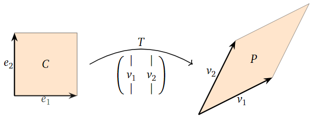
Similarly, for \(n=3\), we can think of \(T\) transforming the unit cube \(C\) int a parallelepiped \(P\) determined by \(\vec v_1, \vec v_2 \text{and} \vec v_3\).
In general, since the unit cube has volume \(1\) and its image has volume \(|\det(A)|\), the transformation \(T\) scales the volume of the cube by a factor of \(|\det(A)|\). Summarizing:
If \(A\) is an \(n\times n\) matrix with corresponding matrix transformation \(T\colon\mathbb{R}^n \to\mathbb{R}^n \text{,}\) and if \(C\) is the unit cube in \(\mathbb{R}^n \text{,}\) then the volume of \(T(C)\) is \(|\det(A)|.\)
The notation \(T(S)\) means the image of the region \(S\) under the transformation \(T\). That is,
\[ T(S) = \bigl\{T(x)\mid x \text{ in } S\bigr\}. \nonumber \]
In fact, \(T\) scales the volume of any region in \(\mathbb{R}^n \) by the same factor, even for curvy regions.
The following theorem follows directly from Theorem 3.4.2 in section 3.4.
Let \(T\colon\mathbb{R}^n \to\mathbb{R}^n \) be a linear transformation with induced matrix \(A\). If \(S\) is any region in \(\mathbb{R}^n \text{,}\) then
\[ \text{vol}(T(S))=|\det(A)|\cdot\text{vol}(S). \nonumber \]
This page titled 5.2: The Matrix of a Linear Transformation I was last modified on Thu, 10 Apr 2025 05:35:55 GMT and is shared under a CC BY 4.0 license and was authored, remixed, and/or curated by Doli Bambhania, Fatemeh Yarahmadi, and Bill Wilson.
The book could not be loaded just now.