Opening the book…
- Model and solve first-order differential equations in real-world applications involving mixture.
- Analyze and solve mixture problems to determine the concentration and quantity of substances over time.
In this section we will look at some simple applications which are modeled with first order differential equations. We will begin with simple rational model of mixture problem in a single tank.
Mixture problems often occur in a first course on differential equations as examples of first order differential equations. In such problems we consider a tank of brine, water containing a specific amount of salt with pure water entering and the mixture leaving, or the flow of a pollutant into, or out of, a lake. The goal is to predict the amount of salt, or pollutant, at some later time.
In general one has a rate of flow of some concentration of mixture entering a region and a mixture leaving the region. The goal is to determine how much stuff is in the region at a given time. This is governed by the equation
Rate of change of substance \(=\) Rate In \(-\) Rate Out.
The rates are not often given. One is generally given information about the concentration and flow rates in and out of the system. If one pays attention to the dimension and sketches the situation, then one can write out this rate equation as a first order differential equation. We consider a simple example.
A 50 gallon tank of pure water has a brine mixture with concentration of 2 pounds per gallon entering at the rate of 5 gallons per minute. At the same time the well-mixed contents drain out at the rate of 5 gallons per minute. Find the amount of salt in the tank at time \(t \). In all such problems one assumes that the solution is well mixed at each instant of time. See Figure \(\PageIndex{1}\) for an illustration of the problem.

Solution
Let \(x(t)\) be the amount of salt at time \(t\). Then the rate at which the salt in the tank increases is due to the amount of salt entering the tank less that leaving the tank. To figure out these rates, one notes that \(d x / d t\) has units of pounds per minute. The amount of salt entering per minute is given by the product of the entering concentration times the rate at which the brine enters. This gives the correct units:
\[\left(2 \dfrac{\text { pounds }}{\text { gal }}\right)\left(5 \dfrac{\text { gal }}{\text { min }}\right)=10 \dfrac{\text { pounds }}{\text { min }} . \nonumber \]
Similarly, one can determine the rate out as
\[\left(\dfrac{x \text { pounds }}{50 \text { gal }}\right)\left(5 \dfrac{\text { gal }}{\text { min }}\right)=\dfrac{x}{10} \dfrac{\text { pounds }}{\text { min }} . \nonumber \]
Thus, we have
\[\dfrac{d x}{d t}=10-\dfrac{x}{10} \nonumber \]
This equation is solved using the methods for linear first order equations. The integrating factor is \(\mu=e^{x / 10}\), leading to the general solution
\[x(t)=100+A e^{-t / 10} \nonumber \]
Using the initial condition, one finds the particular solution
\[x(t)=100\left(1-e^{-t / 10}\right) \nonumber \]
Often one is interested in the long time behavior of a system. In this case we have that \(\lim _{t \rightarrow \infty} x(t)=100 \space \mathrm{lb}\). This makes sense because 2 pounds per galloon enter during this time to eventually leave the entire 50 gallons with this concentration. Thus,
\[50 \space \mathrm{gal} \times 2 \dfrac{\mathrm{lb}}{\mathrm{gal}}=100 \space \mathrm{lb} \nonumber \]
A tank initially contains 40 pounds of salt dissolved in 600 gallons of water. Starting at \(t_0 = 0\), water that contains 1/2 pound of salt per gallon is poured into the tank at the rate of 4 gal/min and the mixture is drained from the tank at the same rate (see Figure 2.4.2 ).
- Find a differential equation for the quantity \(Q(t)\) of salt in the tank at time \(t > 0\), and solve the equation to determine \(Q(t)\).
- Find \(\lim_{t\to\infty}Q(t)\).
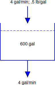
Solution a
To find a differential equation for \(Q\), we must use the given information to derive an expression for \(Q'\). But \(Q'\) is the rate of change of the quantity of salt in the tank changes with respect to time; thus, if rate in denotes the rate at which salt enters the tank and rate out denotes the rate by which it leaves, then
\[\label{eq:4.2.5} Q' = \mbox{rate in}-\mbox{rate out}.\]
The rate in is
\[\left({1\over 2}\ \mbox{lb/gal}\right) \times (4\ \mbox{gal/min}) = 2\ \mbox{lb/min}.\nonumber\]
Determining the rate out requires a little more thought. We’re removing 4 gallons of the mixture per minute, and there are always 600 gallons in the tank; that is, we are removing \(1/150\) of the mixture per minute. Since the salt is evenly distributed in the mixture, we are also removing \(1/150\) of the salt per minute. Therefore, if there are \(Q(t)\) pounds of salt in the tank at time \(t\), the rate out at any time \(t\) is \(Q(t)/150\). Alternatively, we can arrive at this conclusion by arguing that
\[\begin{align*} \mbox{rate out} & = (\mbox{concentration})\times(\mbox{rate of flow out}) \\[5pt] &= (\mbox{lb/gal})\times(\mbox{gal/min})\\[4pt] &= {Q(t)\over600} \times 4 \\[4pt] &={Q(t)\over150}. \end{align*}\nonumber \]
We can now write Equation (2.4.1) as
\[Q' = 2-{Q\over 150}. \nonumber\]
This first order equation can be rewritten as
\[Q'+{Q\over 150} = 2. \nonumber\]
Since \(e^{-t/150}\) is a solution of the complementary equation, the solutions of this equation are of the form \(Q=ue^{-t/150}\), where \(u'e^{-t/150}=2\), so \(u'=2e^{t/150}\). Hence,
\[u = 300e^{t/150}+c, \nonumber\]
so
\[\label{eq:4.2.6} Q=ue^{-t/150}=300+ce^{-t/150}\]
Since \(Q(0)=40\), \(c=-260\); therefore,
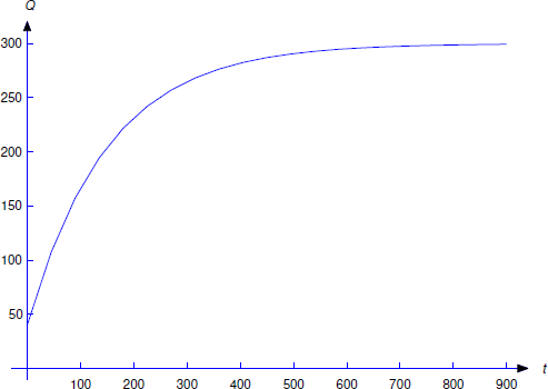
\[Q=300-260e^{-t/150}.\nonumber\]
See Figure 2.4.3 for a graph of the solution.
Solution b
From Equation (2.4.2), we see that that \(\lim_{t \to \infty}Q(t)=300\) for any value of \(Q(0)\). This is intuitively reasonable, since the incoming solution contains 1/2 pound of salt per gallon and there are always 600 gallons of water in the tank.
A 500-liter tank initially contains 10 g of salt dissolved in 200 liters of water. Starting at \(t_0=0\), water that contains 1/4 g of salt per liter is poured into the tank at the rate of 4 liters/min and the mixture is drained from the tank at the rate of 2 liters/min ( see Figure 2.4.4 ). Find a differential equation for the quantity \(Q(t)\) of salt in the tank at time \(t\) prior to the time when the tank overflows and find the concentration \(K(t)\) (g/liter) of salt in the tank at any such time.
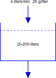
Solution
We first determine the amount \(W(t)\) of solution in the tank at any time \(t\) prior to overflow. Since \(W(0) = 200\) and we are adding 4 liters/min while removing only 2 liters/min, there’s a net gain of 2 liters/min in the tank; therefore,
\[W(t) = 2t+200.\nonumber\]
Since \(W(150)=500\) liters (capacity of the tank), this formula is valid for \(0 \le t \le 150\).
Now let \(Q(t)\) be the number of grams of salt in the tank at time \(t\), where \(0 \le t \le 150\). As in Example 2.4.2
\[\label{eq:4.2.7} Q' = \mbox{rate in}-\mbox{rate out}.\]
The rate in is
\[\label{eq:4.2.8} \left({1\over 4}\ \mbox{g/liter}\,\right) \times (4\ \mbox{liters/min}\,) = 1\ \mbox{g/min}.\]
To determine the rate out, we observe that since the mixture is being removed from the tank at the constant rate of 2 liters/min and there are \(2t+200\) liters in the tank at time \(t\), the fraction of the mixture being removed per minute at time \(t\) is
\[{2\over 2t+200} = {1\over t+100}.\nonumber\]
We’re removing this same fraction of the salt per minute. Therefore, since there are \(Q(t)\) grams of salt in the tank at time \(t\),
\[\label{eq:4.2.9} \mbox{rate out} = {Q(t)\over t+100}.\]
Alternatively, we can arrive at this conclusion by arguing that
\[\begin{array}{lcl} \mbox{rate out} & = & (\mbox{concentration})\times(\mbox{rate of flow out}) =(\mbox{g/liter})\times(\mbox{liters/min})\\[10pt] &=&{Q(t)\over2t+200}\times 2={Q(t)\over t+100}. \end{array} \nonumber \]
Substituting Equation (2.4.4) and Equation (2.4.5) into Equation (2.4.3) yields
\[\label{eq:4.2.10} Q'=1-{Q\over t+100},\quad \text{so} \quad Q'+{1\over t+100} Q=1.\]
By separation of variables, \(1/(t+100)\) is a solution of the complementary equation, so the solutions of Equation (2.4.6) are of the form
\[Q={u\over t+100}, \quad \text{where} \quad {u'\over t+100 }=1, \quad \text{so} \quad u'=t+100.\nonumber\]
Hence,
\[\label{eq:4.2.11} u = {(t+100)^2\over 2}+c.\]
Since \(Q(0)=10\) and \(u=(t+100)Q\), Equation (2.4.7) implies that
\[(100)(10) = {(100)^2\over 2}+c,\nonumber\]
so
\[c=100(10)-{(100)^2\over 2} =-4000\nonumber\]
and therefore
\[u = {(t+100)^2\over 2} -4000.\nonumber\]
Hence,
\[Q = {u\over t+100}= {t+100\over 2}-{4000\over t+100}.\nonumber\]
Now let \(K(t)\) be the concentration of salt at time \(t\). Then
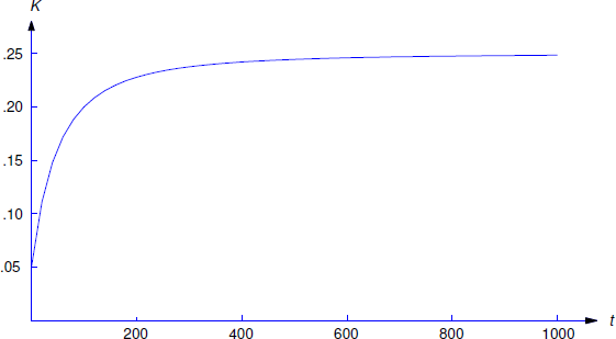
\[K(t) = {1\over 4}-{2000\over(t+100)^2}\nonumber\]
This is shown in Figure 2.4.5 .
This page titled 2.4: Mixing Problems was last modified on Sun, 31 Aug 2025 06:13:59 GMT and is shared under a CC BY-NC-SA 3.0 license and was authored, remixed, and/or curated by Vinh Kha Nguyen, Neelam R. Shukla, and Fatemeh Yarahmadi via source content that was edited to the style and standards of the LibreTexts platform.
The book could not be loaded just now.