Opening the book…
- Use the derivative property of the Laplace transform to evaluate the Laplace transform \({\cal L}\left(t^nf(t)\right)\).
- Solve initial value problems using Laplace transforms, inverse of Laplace transforms, and the derivative property of the Laplace transform.
- Use the Laplace transform to solve linear models such as Newton's Law of Cooling and mass/spring systems.
Derivatives of a Transform
In this section, we will explore how to find the Laplace transform of a function \(f(t)\) that is multiplied by a monomial \(t^n\).
Let \({\cal L}\left(f(t)\right)=F(s)\) and \(n=1, 2, \dots\). Suppose that the order of differentiation and integration can be interchanged. Then
\[{\cal L}\left(t^nf(t)\right)=(-1)^n\dfrac{d^n}{ds^n}{\cal L}\left(f(t)\right)=(-1)^nF(s) \quad \mbox{ for all } n.\label{derivative} \]
- Proof by Mathematical Induction
-
Let \(n=1\), then \[{\cal L}\left(tf(t)\right)= \int_0^\infty e^{-st}t f(t)\,dt =- \int_0^\infty {\partial \over\partial s}\left(e^{-st} f(t)\right)\,dt=-\frac{d}{ds} \int_0^\infty e^{-st} f(t)\,dt=-F(s)\nonumber\]
Then the result in \ref{derivative} holds for \(n=1\).
Assume that \[{\cal L}\left(t^kf(t)\right)= (-1)^k\dfrac{d^k}{ds^k}{\cal L}\left(f(t)\right)=(-1)^kF(s) \label{assumption}\]
holds true for \(n=k\).
Then, for \(n=k+1\), we have
\[{\cal L}\left(t^{k+1}f(t)\right)= \int_0^\infty e^{-st}t^{k+1} f(t)\,dt =- \int_0^\infty {\partial \over\partial s} \left(e^{-st} t^kf(t)\right)\,dt=-\frac{d}{ds} \int_0^\infty e^{-st}t^k f(t)\,dt={\cal L}\left(t^kf(t)\right)\nonumber\]
Since \({\cal L}\left(t^kf(t)\right)=(-1)^kF(s) \) by assumption \ref{assumption}, then
\[{\cal L}\left(t^{k+1}f(t)\right)= -\frac{d}{ds} \left((-1)^kF(s)\right)=(-1)^{k+1}\dfrac{d^{k+1}}{ds^{k+1}}{\cal L}\left(f(t)\right)=(-1)^{k+1}F(s) \nonumber\]
Then the result in \ref{derivative} holds for \(n=k+1\).
Therefore, \[{\cal L}\left(t^nf(t)\right)=(-1)^n\dfrac{d^n}{ds^n}{\cal L}\left(f(t)\right)=(-1)^nF(s) \quad \mbox{ for all } n\nonumber\]
by mathematical induction.
Evaluate the following the Laplace transforms.
a) \({\cal L}\left(t \sin(2t)\right)\)
b) \({\cal L}\left(t^2 e^{4t}\right)\)
Solution
a) Using Theorem \ref{derivative} with \(n=1\) and \(f(t)=\sin(2t)\),
\[{\cal L}\left(t \sin(2t)\right)=-\dfrac{d}{ds}{\cal L}\left(\sin(2t)\right)=-\dfrac{d}{ds}\left(\dfrac{2}{s^2+4}\right)=\dfrac{4s}{(s^2+4)^2}\nonumber\]
b) Using Theorem \ref{derivative} with \(n=2\) and \(f(t)=e^{4t}\),
\[{\cal L}\left(t^2 e^{4t}\right)=(-1)^2\dfrac{d^2}{ds^2}{\cal L}(e^{4t})=\dfrac{d^2}{ds^2}\left(\dfrac{1}{s-4}\right)\nonumber\]
\[=\dfrac{d}{ds}\left(\dfrac{d}{ds}(s-4)^{-1}\right)=\dfrac{d}{ds}(-(s-4)^{-2})=\dfrac{2}{(s-4)^3}\nonumber\]
Linear Models with the Laplace Transform
In chapters 3, we solved linear models of first-order differential equations, such as applications of growth and decay, Newton's Law of Cooling, and mixing problems, while in chapter 5, we solved linear models of second-order differential equations representing simple harmonic motion. These problems can also be solved using Laplace transforms.
Netwon's Law of Cooling
Recall that Newton’s law of cooling states that the rate of change of an object’s temperature is proportional to the difference between its own temperature and the ambient temperature (i.e., the temperature of its surroundings). If we let \(T(t)\) represent the temperature of an object as a function of time with initial temperature \(T_0\), then Newton’s law of cooling can be written in the form
\[ \dfrac{dT}{dt}=k(T−T_s) \label{newton} \]
with \(T(0)=T_0\), where \(k\) is a constant that needs to be either given or determined in the context of the problem.
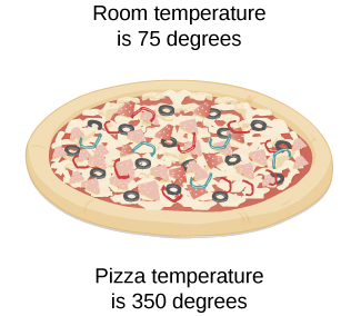
A pizza is removed from the oven after baking thoroughly, and the temperature of the oven is \(350°F.\) The temperature of the kitchen is \(75°F\). We would like to wait until the temperature of the pizza reaches \(300°F\) before cutting and serving it (Figure \(\PageIndex{3}\)). If the cooling constant \(k=-0.01\), how much longer will we have to wait?
Solution
The ambient temperature (surrounding temperature) is \(75°F\), so \(T_s=75\) and the cooling constant is \(k=-0.01\). The temperature of the pizza when it comes out of the oven is \(350°F\), which is the initial temperature, so \(T_0=350\). Therefore Equation \ref{newton} becomes
\[\dfrac{dT}{dt}=-0.01(T−75)\quad \quad \text{with} \quad \quad T(0)=350\nonumber \]
which can be rewritten as
\[T'+0.01T=0.75 \quad \quad \text{with} \quad \quad T(0)=350\label{eq:7.4.1} \]
Taking Laplace transforms of both sides of the differential equation in Equation \ref{eq:7.4.1} yields
\[{\cal L}( T'+0.01T)={\cal L}(0.75)={0.75\over s},\nonumber \]
which we rewrite as
\[\label{eq:7.4.2} {\cal L}(T')+0.01{\cal L}(T)={0.75\over s}. \]
Now denote \({\cal L}(T)=Y(s)\), then
\[{\cal L}(T')=sY(s)-T(0)=sY(s)-350\nonumber \]
Substituting from the equation into Equation \ref{eq:7.4.2} yields
\[sY(s)-350+0.01Y(s)={0.75\over s}.\nonumber \]
Therefore
\[(s+0.01)Y(s)={0.75\over s}+350.\nonumber \]
Solving for \(Y(s)\) yields
\[Y(s)={0.75+350s\over s(s+0.01)}.\nonumber \]
Partial fraction decompositions yields the partial fraction expansion
\[Y(s)={75\over s}+{275\over s+0.01},\nonumber \]
and taking the inverse transform we get
\[{\cal L}^{-1}(Y(s))=75{\cal L}^{-1}\Big({1\over s}\Big)+275{\cal L}^{-1}\Big({1\over s+0.01}\Big),\nonumber \]
Therefore the solution of Equation \ref{eq:7.4.1} over the interval \([0, \infty)\) is
\[T(t)=75+275e^{-0.01t}\nonumber \]
We now need to find how long we need to wait till the temperature of the pizza reaches \(300°F\). Solving for \(t\), we get
\[300=75+275e^{−0.01t}\nonumber \]
\[225=275e^{−0.01t}\nonumber \]
\[e^{−0.01t}=\dfrac{225}{275}=\dfrac{9}{11}\nonumber \]
\[\ln e^{−0.01t}=\ln\dfrac{9}{11}\nonumber \]
\[−0.01t=\ln\dfrac{9}{11}\nonumber \]
\[t=−\dfrac{1}{0.01}\ln\dfrac{9}{11}≈20.1.\nonumber \]
Therefore we need to wait about \(20\) minutes.
Simple Harmonic Motion
Recall that we model systems with simple harmonic motion where an external force is acting on the system with the nonhomogeneous differential equation
\[mx″+bx′+kx=f(t), \nonumber \]
where the external force is represented by the \(f(t)\) term.
We will use Laplace transforms to solve these problems when subject to an initial position \(x(0)\) and and initial velocity \(x'(0)\).
An object with mass \(20\) kg is attached to a spring with constant \(k=80\) kg/m and subjected to an external force \(f(t)=-1200\cos(2t)\). The object begins at rest in its equilibrium position. Use the Laplace transform to find its displacement for \(t>0\).
Solution
Notice that the system is undamped, so \(b=0\). Therefore, the scenario can be modeled using the nonhomogeneous differential equation
\[20x″+80x=-1200 \cos(2t),\quad \quad \text{with} \quad \quad x(0)=0\quad and \quad x'(0)=0 \label{eq:7.4.3} \]
Taking Laplace transforms of both sides of the differential equation yields
\[{\cal L}( 20x″+80x)={\cal L}\left(-1200\cos(2t)\right),\nonumber \]
which we rewrite as
\[\label{eq:8.3.15} 20{\cal L}(x'')+80{\cal L}(x)=-1200{\cal L}\left(\cos(4t)\right)={-1200s\over s^2+4}. \]
Now denote \({\cal L}(x)=X(s)\), then
\[{\cal L}(x')=sX(s)-x(0)=sX(s)\nonumber \]
and
\[{\cal L}(x'')=s^2X(s)-x'(0)-sx(0)=s^2X(s).\nonumber \]
Substituting from the last two equations into Equation \ref{eq:7.4.3} yields
\[20s^2X(s)+80X(s)={-1200s\over s^2+4}.\nonumber \]
Therefore
\[20(s^2+4)Y(s)={-1200s\over s^2+4}.\nonumber \]
Solving for \(X(s)\) yields
\[X(s)={-1200 s\over 20(s^2+4)^2}={-60s\over (s^2+4)^2}.\nonumber \]
Taking the inverse transform we get
\[{\cal L}^{-1}(X(s))=-60{\cal L}^{-1}\Big({s\over (s^2+4)^2}\Big),\nonumber \]
We just saw in example 7.4.1. that \({\cal L}(t\sin(2t))={4s\over (s^2+4)^2}\). Then
\[x(t)={-60\over4}{\cal L}^{-1}\Big({4s\over (s^2+4)^2}\Big)=-15t\sin(2t)\nonumber \]
is the solution of Equation \ref{eq:7.4.3} over the interval \([0, \infty)\).
In general, for \({\cal L}\left(t^nf(t)\right)=(-1)^nF(s)\) from Theorem \ref{derivative}, we can deduce \({\cal L}^{-1}(F(s))\) as listed below.
| Inverse Laplace Transforms |
| \[{\cal L}^{-1}\left({1\over (s-a)^2}\right)=te^{at}\nonumber\] |
| \[{\cal L}^{-1}\left({n!\over (s-a)^{n+1}}\right)=t^ne^{at}\nonumber\] |
| \[{\cal L}^{-1}\left({2ks\over (s^2+k^2)^{2}}\right)=t\sin(kt)\nonumber\] |
| \[{\cal L}^{-1}\left({s^2-k^2\over (s^2+k^2)^{2}}\right)=t\cos(kt)\nonumber\] |
| \[{\cal L}^{-1}\left({2ks^2\over (s^2+k^2)^{2}}\right)=\sin(kt)+kt\cos(kt)\nonumber\] |
| \[{\cal L}^{-1}\left({2k^3\over (s^2+k^2)^{2}}\right)=\sin(kt)-kt\cos(kt)\nonumber\] |
7.4: Derivatives of Laplace Transforms and Linear Models is shared under a not declared license and was authored, remixed, and/or curated by LibreTexts.
The book could not be loaded just now.