Opening the book…
As stressed in the last chapter, the point of a random variable is to model some sort of quantity, process, or real life phenomenon. Up until now, we have discussed how discrete random variables can be used to model certain quantities; for instance, they can model the total number of successes among \(n\) independent trials or they may model the number of trials until your first success or they may model the number of occurrences of a particular event. However, discrete random variables fall short in the sense that they cannot model every quantity out there in the universe. Specifically, there are certain quantities which are not discrete in nature and thus will require a different type of random variable. The focus of this chapter is to discuss this new type of random variable called a continuous random variable. Essentially, we will have a continuous random variable whenever the quantity we wish to study or model can assume every value along some interval of real numbers. Before we rigorously define a continuous random variable, allow us to concretely understand the shortcomings of a discrete random variable and in doing so, we will motivate the need for a continuous random variable.
- Suppose you wished to model the height of a person. Is height a discrete quantity or a continuous quantity? To be clear, when we say discrete quantity, we mean something along the lines of the random variable assuming the values \(1, 2, 3, 4, \ldots\) and whenever we say continuous, we typically mean that the random variable can assume every value over some interval. Clearly, height is a continuous quantity. Why? Well, if you said that height was discrete then you are (roughly) saying that a person's height can only assume values such as \(1, 2, 3, 4, 5, \ldots\). If we are measuring in inches, then you are saying it is impossible for someone to be 62.34254543... inches and since this may actually happen, this quantity is not discrete. Alternatively, one may think about this another way. Is it possible to grow from 5 feet 2 inches and then immediately become 5 feet 3 inches? No! When you grow, you do not grow discretely. Your body does not say we can only grow in one inch increments. Instead, as you grow from 5 feet 2 inches to 5 feet 3 inches, your height assumes every possible real number from 62 inches to 63 inches and so height must be a continuous quantity.
- Think about the amount of rain that falls when you watch the news. Or better yet, imagine you were measuring the rain fall in your backyard. At some time, \(t_1\), you may have recorded one inch of rain and at a later moment in time, \(t_2\), you may have measured 2 inches of rain. As the rainfall increased from 1 inch to 2 inches, the amount of rain that fell assumed every real number along that interval!
- Yet another example of something that fails to be discrete is the waiting time between events that occur according to a Poisson Process. For instance, let us suppose that the number of earthquakes that occurs follows a Poisson random variable and let us define a random variable \(X\) that models the amount of time that passes between the first and second earthquake. Is \(X\) discrete? Meaning, does the earthquake wait to occur on only integer or rational values of time? Nope! The earthquake can happen at any given instance and so we can think of \(X\) as being continuous on \((0, \infty)\). For more information about waiting times a good idea is to search "Queueing Theory".
- Another example we may consider is what if \(X\) models picking a number at random from the interval \([0,1] = \{ x \in \mathbb{R} ~|~ 0 \leq x \leq 1 \}\). For those with a background in discrete mathematics, you may recognize this to be an uncountably infinite set and thus \(X\) cannot be a discrete random variable since by definition, a discrete random variable takes on at most a countably infinite number of values.
- Finally, consider the amount of miles a car gets per gallon. Since the amount of miles can assume any real number over some interval, \(X\) is a continuous random variable.
In summary, discrete random variables fail to model many quantities and thus a new class of random variables are needed. This class is called continuous random variables.
Definition: We say that a random variable \(X\) has a continuous distribution or that \(X\) is a continuous random variable if there exists a nonnegative function \(f\), defined on the real line, such that for every interval of real numbers, the probability that \(X\) takes a value in the interval is the integral of \(f\) over the interval. We call this nonnegative function, \(f\), the probability density function (pdf) of \(X\).
In terms of a diagram, the above definition is saying the following: suppose we have a continuous random variable \(X\) that has the following probability density function:

If we wish to find \(P (a \leq X \leq b\) then all we have to do is simply integrate \(f\) from \(a\) to \(b\). That is, for a continuous random variable,
\[ P( a \leq X \leq b) = \int_{a}^{b} f(x) ~ dx \] which geometrically represents the area underneath the curve of \(f\) from \(a\) to \(b\) as pictured below:
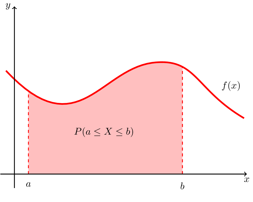
More generally, the above definition is saying \[ P(X \in I) \ = \int_{I} f(x) ~ dx \]. In words, this is saying for any continuous random variable, \(X\) to find the probability that \(X\) belongs to some interval of real numbers, we simply integrate the density function over that interval.
Believe it or not, when it comes to the theory of continuous random variables, we pretty much already know it! Before we explain why, allow us to consider a quick example based on the above definition.
Suppose a random variable \(X\) has the following density:
\(
f(x) =
\begin{cases}
\frac{1}{196} & \text{if} ~ 4 \leq x \leq 200 \\
0 & \text{otherwise} \\
\end{cases}
\)
Find
- \(P(20 \leq X \leq 50)\)
- \(P(X \leq 50) = F(50)\)
- \(P(X = 20)\)
- Answer
-
1. When it comes to continuous random variables, we should always have a picture in mind and so allow us to graph the density function. Doing so yields:

Based off our definition of a continuous random variable, \[ P(X \in I) \ = \int_{I} f(x) ~ dx \nonumber\ \] and so \[ P(20 \leq X \leq 50) = \int_{20}^{50} f(x) ~ dx = \int_{20}^{50} \frac{1}{196} ~ dx = \frac{30}{196} \nonumber \]
2. Again, we must simply integrate over the appropriate region while recalling from calculus how to integrate a piecewise defined function. Hence, we obtain the following: \begin{align*} F(50) = P(X \leq 50) &= \int_{- \infty}^{50} f(x) dx \\ &= \int_{- \infty}^{4} 0 ~ dx && + \int_{4}^{50} \frac{1}{196} ~ dx \\ & = 0 && + \int_{4}^{50} \frac{1}{196} ~ dx \\ & = \frac{46}{196} \end{align*}
3. For this part, we again must integrate \(f\) over the appropriate region. The interval \( \{ X=20 \} \) is simply the single point \(x=20\) and so we have \[ P(X= 20) = \int_{20}^{20} f(x) ~ dx = 0 \nonumber\ \]
The third part of the above problem shows us an extremely important result which is true for all continuous distributions.
Theorem: If \(X\) is a continuous random variable, then \(P(X = a) = 0\).
- Proof:
-
Let \(f\) denote the probability density function of \(X\). Then \(P(X = a) = \int_{a}^{a} fx(x) ~ dx = 0 \).
The formal proof is quite simple and we should recall the intuitive idea of what is happening here. Essentially, to find the probability that \(X\) equals to a single point, by definition, we must integrate over that region which geometrically means find the area underneath the curve. But that region is simply a one-dimensional line and the area underneath the curve of any one-dimensional line is always 0. So again, for any continuous random variable, the probability that the random variable equals a single value is always zero. We only start to get nonzero probabilities whenever we integrate \textit{over a (non-zero) region}.
As a consequence of the above discussion, please note that unlike discrete random variables, when it comes to finding probabilities for continuous random variables, it does not matter if the endpoints of an interval are included or not since the probability \(X\) equals to these values would be zero. Let us verify this claim in the next example.
Suppose a random variable \(X\) has the following density:
\(
f(x) =
\begin{cases}
\frac{1}{196} & \text{if} ~ 4 \leq x \leq 200 \\
0 & \text{otherwise} \\
\end{cases}
\)
Find \(P( 20 < X < 50)\).
- Answer
-
To find \(P( 20 < X < 50)\( we simply integrate \(f\) over this region.
\begin{align*} P(20 < X < 50) &= \int_{20}^{50} f(x) ~ dx \\ &= \int_{20}^{50} \frac{1}{196} ~ dx \\ &= \frac{30}{196} \end{align*}
However, some students tend to object to this computation. They often feel like the limits of integration are incorrect even though they are not. Thus, allow me to argue this another way.
\begin{align*}
\{ 20 \leq X \leq 50 \} &= \{ X = 20 \} \cup \{ 20 < X < 50 \} \cup \{ X = 50 \} \\
\rightarrow P(20 \leq X \leq 50) &= P(X=20) + P( 20 < X < 50) + P(X = 50) \\
\rightarrow P(20 \leq X \leq 50) &= 0 + P( 20 < X < 50) + 0 \\
\rightarrow P(20 \leq X \leq 50) &= P( 20 < X < 50) \\
\rightarrow \frac{30}{196} &= P( 20 < X < 50)
\end{align*}
Earlier we said when it comes to the theory of continuous random variables, we pretty much already know the theory. We are now in a position to say why. Informally, we make the following comment:
Loosely speaking, if we replace the summation sign in the theory for discrete random variables with an integral, then we obtain the theory for continuous random variables.
More formally, we present the following chart which gives a summary of the theory required for discrete random variables and continuous random variables. In doing so, we see how similar the two types of random variables are.
| Discrete Random Variables | Continuous Random Variables |
|---|---|
| \(f(x)\) is called the probability mass function (pmf) | \(f(x)\) is called the probability density function (pdf) |
| \(f(x) \geq 0\) for all \(x\) | \(f(x) \geq 0\) for all \(x\) |
| \( \sum_{\text{all} ~ x} f(x) = 1\) | \( \int_{\text{all} ~ x} f(x) ~ dx= 1\) or equivalently \( \int_{- \infty}^{\infty} f(x) ~ dx = 1 \) |
| \( P(X \in A) \ = \sum_{\text{all} ~ x \in A} f(x) \) | \( P(X \in I) \ = \int_{I} f(x) ~ dx \) |
| The cumulative distribution function is typically denoted by \(F\) | The cumulative distribution function is typically denoted by \(F\) |
| \( \displaystyle F(x) = P(X \leq x) = \sum_{\text{all values less than or equal to} ~ x } f(x) \) | \( \displaystyle F(x) = P(X \leq x) = \displaystyle \int_{\text{all values less than or equal to} ~ x } f(t) ~ dt = \int_{- \infty}^{x} f(t) ~ dt \) |
| \( pmf \xrightarrow[summing]{} cdf \) | \( pdf \xrightarrow[integrating]{} cdf \) |
| \( cdf \xrightarrow[subtracting]{} pdf \) | \( cdf \xrightarrow[differentiating]{} pdf \) |
| \( \mathbb{E}[X] = \sum_{\text{all} ~ x} xf(x) \) | \( \mathbb{E}[X] = \int_{\text{all} ~ x} xf(x) ~ dx = \int_{- \infty}^{\infty} f(x) ~ dx \) |
| LOTUS: \( \mathbb{E}[g(X)] = \sum_{\text{all} ~x } g(x)f(x) \) | LOTUS: \( \mathbb{E}[g(X)] = \int_{\text{all} ~x } g(x)f(x) ~ dx = \int_{- \infty}^{\infty} g(x)f(x) ~ dx \) |
| \( \mathbb{V}ar[X] = \mathbb{E}[X^2] - \bigg( \mathbb{E}[X] \bigg)^2 \) | \( \mathbb{V}ar[X] = \mathbb{E}[X^2] - \bigg( \mathbb{E}[X] \bigg)^2 \) |
| \( SD[X] = \sqrt{\mathbb{V}ar[X]} \) (again we only care for the positive square root) | \( SD[X] = \sqrt{\mathbb{V}ar[X]} \) (again we only care for the positive square root) |
Notice a fundamental difference between the probability mass function and the probability density function. In the probability mass function, we obtain probabilities by summing over the appropriate values of \(x\) when plugged into the function, \(f\). However, with a probability density function, we obtain probabilities by integrating the function over the appropriate region. Thus we should NEVER plug a value into a density function and think that the value obtained is the corresponding probability. For instance, with regards to Example 1, the following would be incorrect: \(P(X=20) = f(20) = \frac{1}{196} \). We are only allowed to plug in if we have a discrete random variable!
In short, plugging in values into a density does not yield a probability. Instead, we only obtain a probability once we integrate the density over the appropriate interval.
Once you know the above chart, you can pretty much work with any continuous random variable. Let us touch upon every aspect of that chart by considering the following examples.
Suppose \(X\) has the following density: \(
f(x) =
\begin{cases}
cx^2 & \text{if} ~ 2 \leq x \leq 4 \\
0 & \text{otherwise} \\
\end{cases}
\)
1) Find the value of \(c\).
2) \( P( 2 \leq X \leq 3) \).
3) Is \( P( -10 \leq X \leq 3) = P( 2 \leq X \leq 3) \) ?
4) Find the cumulative distribution function of \(X\).
5) Using the cumulative distribution function of \(X\) find \( P( 2 \leq X \leq 3) \).
6) Find \( \mathbb{E}[X] \).
7) Find \( \mathbb{V}ar[X] \).
- Answer
-
1) We will first walk through the full details of this problem and then at the end we will simplify it. If this was a discrete random variable, how would we find the value of \(c\)? Think back to the homework or our review sheet. To find the value of \(c\), we would impose the condition that \( \sum_{all ~ x} f(x) = 1 \). According to our chart, what is the analogous property for the continuous case? The analogous property is that \( \int_{- \infty}^{\infty} f(x) ~ dx = 1 \). We impose this condition and we may easily find \(c\).
\begin{align*}
\int_{- \infty}^{\infty} f(x) ~ dx &= 1
\end{align*}Recall from calculus that since \(f\) is a piecewise defined function, we have to break up the integral over each piece:
\begin{align*}
\int_{- \infty}^{\infty} f(x) ~ dx &= 1 \\
\int_{- \infty}^{2} 0 ~ dx + \int_{2}^{4} cx^2 ~ dx + \int_{4}^{\infty} 0 ~ dx &= 1
\end{align*}
We see that the first and third integrals are simply zero. Thus we have the following calculation:\begin{align*}
\int_{- \infty}^{\infty} f(x) ~ dx &= 1 \\
\int_{- \infty}^{2} 0 ~ dx + \int_{2}^{4} cx^2 ~ dx + \int_{4}^{\infty} 0 ~ dx &= 1 \\
\int_{2}^{4} cx^2 ~ dx &= 1 \\
c \int_{2}^{4} x^2 ~ dx &= 1 \\
c \bigg[ \frac{1}{3}x^3 \Biggr|_{2}^{4} \bigg] &= 1 \\
c \bigg[ \frac{64}{3} - \frac{8}{3} \bigg] &= 1 \\
c \bigg[ \frac{56}{3} \bigg] &= 1 \\
c &= \frac{3}{56}
\end{align*}Hence the probability density function is given by
\(
f(x) =
\begin{cases}
\frac{3}{56} x^2 & \text{if} ~ 2 \leq x \leq 4 \\
0 & \text{otherwise} \\
\end{cases}
\)And so the graph of \(f\) looks like the following:

Before we move onto the next part, allow us to make a quick remark which will help us in the future. We said to find the value of \(c\) we must integrate over all \(x\) our function \( f(x) \). When we say over all \( x \), we mean we must integrate from \(-\infty$ to $\infty \). However, recall what we also said earlier: we only start to get nonzero probabilities whenever we integrate over a non-zero region. Thus, to find the value of \(c\) we do not have to really integrate from \( -\infty$ to $\infty \). Instead, we only have to integrate over the values of \(x\) which has a nonzero density! Thus, to start the problem, I could begin by writing
\begin{align*}
\int_{2}^{4} cx^2 ~ dx &= 1
\end{align*} and proceed from there.2) Here, we are asked to find \( P( 2 \leq X \leq 3) \). To find the desired probability, we simply integrate the density over the appropriate region.
\begin{align*}
P(2 \leq X \leq 3) &= \int_{2}^{3} \frac{3}{56} x^2 ~ dx \\
&= \frac{3}{56} \int_{2}^{3} x^2 ~ dx \\
&= \frac{3}{56} \bigg[ \frac{1}{3} x^3 \Biggr|_{2}^{3} \bigg] \\
&= \frac{1}{56} \bigg[ x^3 \Biggr|_{2}^{3} \bigg] \\
&= \frac{1}{56} \bigg[ 27-8 \bigg] \\
&= \frac{19}{56}
\end{align*}3) Recall the density looks like this:
From the picture, we see in finding \( P( -10 \leq X \leq 3) \), the interval from \( [-10, 2] \) does not contribute any probability. Thus, \( P( -10 \leq X \leq 3) \) is indeed the same as \( P( 2 \leq X \leq 3) \).
4) Before we find the cumulative distribution function of \(X\), allow us to discuss the job of a cdf for a continuous random variable. We can think of the cdf of a continuous random variable as the "area so far" function. That is, given some density \(f\), the cdf is the function,\(F\), such that when we plug in some value of \(x\) into \(F\), \(F\) will tell us how much area is underneath the density from the left to the value of \(x\). \\
As a reminder, here is what the probability density function looks like.
Since the function has three pieces, our cumulative distribution function will also have three pieces. One piece will tell us the "area so far" when \( x < 2 \). The other piece will tell us the "area so far" when \(2 \leq x \leq 4\). The last piece will tell us the "area so far" when \(x > 4\). That is, we will have the following:
\[
F(x) =
\begin{cases}
????? & \text{if} ~ x < 2 \\
????? & \text{if} ~ 2 \leq x \leq 4 \\
????? & \text{if} ~ x > 4 \\
\end{cases}
\nonumber\ \]Two of these pieces are easy to find. Notice when \( x < 2 \) what is \( F(x) = P(X \leq x) \) ? Well when \( x < 2 \), to find \( F(x) = P(X \leq x) \) we have to integrate from \(- \infty \) to \( x \). Clearly this integral will equal 0 since we have "no area" from \( - \infty \) to any \( x <2 \).
Additionally, when \( x > 4 \) what is \(F(x) = P(X \leq x)\)? Well when \( x > 4 \), to find \( F(x) = P(X \leq x) \) we have to integrate from \(- \infty \) to \( x \). Clearly this integral will equal 1 since we have covered the entire nonzero portion of the density. Moreover, in part 1, we said
\begin{align*}
\int_{2}^{4} f(x) ~ dx &= 1 \\
\end{align*}At this point, we are almost done. We know the following:
\[
F(x) =
\begin{cases}
0 & \text{if} ~ x < 2 \\
????? & \text{if} ~ 2 \leq x \leq 4 \\
1 & \text{if} ~ x > 4 \\
\end{cases} \nonumber\ \]All that remains is to investigate what happens to the cdf, \( F(x) \) when \( 2 \leq x \leq 4 \). To do this, we apply the rule from our chart:
\begin{align*}
F(x) = \int_{- \infty}^{x} f(t) ~ dt
\end{align*}Before we apply this rule, allow us to be reminded of what we are searching for here. We are asking if \( x\) is some value between 2 and 4, what is the area underneath the function up until \( x\) ?
We see in the formula,
\begin{align*}
F(x) = \int_{- \infty}^{x} f(t) ~ dt
\end{align*}We need \( f(t) \). Since
\[ f(x) =
\begin{cases}
\frac{3}{56} x^2 & \text{if} ~ 2 \leq x \leq 4 \\
0 & \text{otherwise} \\\end{cases} \nonumber\ \]then
\[ f(t) =
\begin{cases}
\frac{3}{56} t^2 & \text{if} ~ 2 \leq t \leq 4 \\
0 & \text{otherwise} \\\end{cases} \nonumber\ \]This is just our density with the variable \(x\) being replaced by \(t\). We now apply the formula in our chart and recall that we only care about the regions which have a non-zero density:
\begin{align*}
F(x) &= \int_{- \infty}^{x} f(t) ~ dt \\
&= \int_{2}^{x} f(t) ~ dt \\
&= \int_{2}^{x} \frac{3}{56} t^2 ~ dt \\
&= \frac{3}{56} \int_{2}^{x} t^2 ~ dt \\
&= \frac{3}{56} \bigg[ \frac{1}{3} t^3 \Biggr|_{2}^{x} \bigg]\\
&= \frac{1}{56} \bigg[ t^3 \Biggr|_{2}^{x} \bigg] \\
&= \frac{1}{56} \bigg[ x^3 - 8 \bigg] \\
&= \frac{x^3 - 8}{56} \\
&= \frac{1}{56} (x^3 - 8)
\end{align*}Putting these three pieces together yields the following:
\[
F(x) =
\begin{cases}
0 & \text{if} ~ x < 2 \\
\frac{1}{56} (x^3 - 8) & \text{if} ~ 2 \leq x \leq 4 \\
1 & \text{if} ~ x > 4 \end{cases} \nonumber\ \]There are two important observations we should make note of. First, notice when we differentiate the cumulative distribution function, we get back the probability density function! Secondly, notice that the equality at each endpoint does not matter. That is, you could write your answer as
\[
F(x) =
\begin{cases}
0 & \text{if} ~ x \leq 2 \\
\frac{1}{56} (x^3 - 8) & \text{if} ~ 2 < x < 4 \\
1 & \text{if} ~ x \geq 4 \\ \end{cases} \nonumber\ \]and this would still be correct. This stems from the fact that the probability at any single point is zero.
Although this was not asked, here is what the cumulative distribution function looks like if you were to graph it:

5) Again, consider the graph of the density function:
We wish to find \( P( 2 \leq X \leq 3) \). Notice that the area underneath \(f\) from 2 to 3 is precisely the area up to 3 minus the area up to 2. Hence \[ P( 2 \leq X \leq 3) = F(3) - F(2) = \frac{19}{56} - 0 = \frac{19}{59} \).
6) \begin{align*}
\mathbb{E}[X] &= \int_{- \infty}^{\infty} xf(x) ~ dx \\ \\
&= \int_{2}^{4} xf(x) ~ dx \\
&= \int_{2}^{4} x \times \frac{3}{56} x^2 ~ dx \\
&= \int_{2}^{4} \frac{3}{56} x^3 ~ dx \\
&= \frac{45}{14}
\end{align*}7) To find \( \mathbb{V}ar[X] \), we use the formula \( \mathbb{V}ar[X] = \mathbb{E}[X^2] - ( \mathbb{E}[X] )^2 \). We already found \( \mathbb{E}[X] \) above. Let us use The Law of the Unconscious Statistician to find \( \mathbb{E}[X^2]\).
\begin{align*}
\mathbb{E}[X^2] &= \int_{- \infty}^{\infty} x^2 f(x) ~ dx \\ \\
&= \int_{2}^{4} x^2 f(x) ~ dx \\
&= \int_{2}^{4} x^2 \times \frac{3}{56} x^2 ~ dx \\
&= \int_{2}^{4} \frac{3}{56} x^4 ~ dx \\
&= \frac{372}{35}
\end{align*}Putting everything together, we obtain
\begin{align*}
\mathbb{V}ar[X] &= \mathbb{E}[X^2] - ( \mathbb{E}[X] )^2 \\
&= \frac{372}{35} - \bigg( \frac{45}{14} \bigg)^2 \\
&= \frac{291}{980}
\end{align*}
Suppose the random variable \(X\) has the following probability density function:
\(
f(x) =
\begin{cases}
ce^{- 10x} & \text{if} ~ x >0 \\
0 & \text{otherwise} \\
\end{cases}
\)
- Find the value of \(c\).
- Find \(P( 0 \leq X \leq 1) \).
- Find the cumulative distribution function of \(X\).
- Find \(\mathbb{E}[X]\).
- Answer
-
1. Similar to the last problem, we impose the condition that \( \int_{- \infty}^{\infty} f(x) ~ dx = 1 \) in order to find \(c\).
\begin{align*}
\int_{- \infty}^{\infty} f(x) ~ dx &= 1 \\
\int_{- \infty}^{0} 0 ~ dx + \int_{0}^{\infty} ce^{-10x} ~ dx &= 1 \\
\int_{0}^{\infty} ce^{-10x} ~ dx &= 1 \\
c \int_{0}^{\infty} e^{-10x} ~ dx &= 1 \\
c \lim_{t \rightarrow \infty} \bigg[ \int_{0}^{t} e^{-10x} ~ dx \bigg] &= 1 \\
c \lim_{t \rightarrow \infty} \bigg[ -\frac{1}{10} e^{-10x} \Biggr|_{0}^{t} \bigg] &= 1 \\
-\frac{c}{10} \lim_{t \rightarrow \infty} \bigg[ e^{-10x} \Biggr|_{0}^{t} \bigg] &= 1 \\
-\frac{c}{10} \lim_{t \rightarrow \infty} \bigg[ e^{-10t} - e^{-10(0)} \bigg] &= 1 \\
-\frac{c}{10} \lim_{t \rightarrow \infty} \bigg[ e^{-10t} - 1 \bigg] &= 1 \\
-\frac{c}{10} \lim_{t \rightarrow \infty} \bigg[ \frac{1}{e^{10t}} - 1 \bigg] &= 1 \\
-\frac{c}{10} \bigg[ 0 - 1 \bigg] &= 1 \\
\frac{c}{10} &= 1 \\
c &= 10
\end{align*}Hence the probability density function is given by
\[
f(x) =
\begin{cases}
10e^{- 10x} & \text{if} ~ x >0 \\
0 & \text{otherwise} \\
\end{cases}
\nonumber\ \]2. Here, we are asked to find $P( 0 \leq X \leq 1)$. To find the desired probability, we simply integrate the density over the appropriate region.
\begin{align*}
P(0 \leq X \leq 1) &= \int_{0}^{1} f(x) ~ dx \\
&= \int_{0}^{1} 10e^{-10x} ~ dx \\
&= -e^{-10x} \Biggr|_{0}^{1} \\
&= -e^{-10} - (-e^0) \\
&= -e^{-10} - (-1) \\
&= 1 - e^{-10}
\end{align*}3. Here is what the density function looks like:

Clearly, when \( x \leq 0, F(x) = 0 \) since we have no area from\( - \infty \) to any \( x \leq 0 \).
So we have the following piecewise defined function:
\[
F(x) =
\begin{cases}
0 & \text{if} ~ x \leq 0 \\
????? & \text{if} ~ x > 0 \\
\end{cases}
\nonumber\ \]To find out what the cdf is when \( x>0 \) we use the rule from our chart. When \( x>0 \) we have the following:
\begin{align*}
F(x) &= \int_{- \infty}^{x} f(t) ~ dt \\
&= \int_{0}^{x} f(t) ~ dt \\
&= \int_{0}^{x} 10e^{-10t} ~ dt \\
&= -e^{-10t} \Biggr|_{0}^{x} \\
&= -e^{-10x} - (-e^{-10(0)}) \\
&= -e^{-10x} - (-1) \\
&= 1 - e^{-10x}
\end{align*}And so we have
\[
F(x) =
\begin{cases}
0 & \text{if} ~ x \leq 0 \\
1 - e^{-10x} & \text{if} ~ x > 0 \\
\end{cases} \nonumber\ \]Notice that as \( x \rightarrow \infty, F(x) \rightarrow 1 \) and also observe that when we differentiate the cumulative distribution function, we get back the probability density function.
4. \begin{align*}
\mathbb{E}[X] &= \int_{- \infty}^{\infty} xf(x) ~ dx \\ \\
&= \int_{- \infty}^{0} xf(x) ~ dx + \int_{0}^{\infty} xf(x) ~ dx \\
&= \int_{- \infty}^{0} x(0) ~ dx + \int_{0}^{\infty} x(10e^{-10x}) ~ dx \\
&= 0 + \int_{0}^{\infty} x(10e^{-10x}) ~ dx \\
&= \int_{0}^{\infty} x(10e^{-10x}) ~ dx & & \text{Improper Integral} \\ &= \lim_{t \rightarrow \infty} \bigg[ \int_{0}^{t} x \times 10e^{-10x} ~ dx \bigg] & & \text{Integration by parts with} ~ u = x, dv = 10e^{-10x} ~ dx \\ &= \lim_{t \rightarrow \infty} \bigg[ -x e^{-10x} \bigg|_{0}^{t} - \int_{0}^{t} - e^{-10x} ~ dx \bigg] \\ &=\lim_{t \rightarrow \infty} \bigg[ (-te^{-10t} + 0) + \int_{0}^{t} e^{-10x} ~ dx \bigg] \\ &= \lim_{t \rightarrow \infty} \bigg[ -te^{-10t} + \bigg( - \frac{1}{10} e^{-10x} \bigg) \bigg|_{0}^{t} \bigg] \\ &= \lim_{t \rightarrow \infty} \bigg[ - \frac{t}{e^{10t}} + \bigg( - \frac{1}{10}e^{-10t} + \frac{1}{10} \bigg) \bigg] \\ &= \lim_{t \rightarrow \infty} \bigg[ - \frac{t}{e^{10t}} - \frac{1}{10}e^{-10t} + \frac{1}{10} \bigg] & & \text{L'Hospital's Rule} \\ &= \frac{1}{10}
\end{align*}
11.1: Continuous Random Variables is shared under a CC BY license and was authored, remixed, and/or curated by LibreTexts.
The book could not be loaded just now.