Opening the book…
In this example we’ll develop a model of Spider-Man swinging from a springy cable of webbing attached to the top of the Empire State Building. Initially, Spider-Man is at the top of a nearby building, as shown in Figure 14.1.
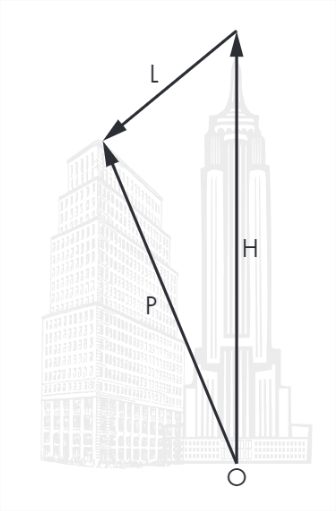 Figure 14.1: Diagram of the initial state for the Spider-Man example
The origin, O, is at the base of the Empire State Building. The vector H represents the position where the webbing is attached to the building, relative to O. The vector P is the position of Spider-Man relative to O. And L is the vector from the attachment point to Spider-Man.
By following the arrows from O, along H, and along L, we can see that
H + L = PSo we can compute L like this:
L = P - HAs an exercise, simulate this system and estimate the parameters that maximize the distance Spider-Man swings.
- Implement a model of this scenario to predict Spider-Man’s trajectory.
- Choose the right time for Spider-Man to let go of the webbing in order to maximize the distance he travels before landing.
- Choose the best angle for Spider-Man to jump off the building, and the best time to let go of the webbing, to maximize range.
Use the following parameters:
- According to the Spider-Man Wiki (https://greenteapress.com/matlab/spider), Spider-Man weighs 76kg.
- Assume his terminal velocity is 60 m/s.
- The length of the web is 100 m.
- The initial angle of the web is 45° to the left of straight down.
- The spring constant of the web is 40 N/m when the cord is stretched and 0 N/m when it’s compressed.
This page titled 14.3: Spider-Man was last modified on Thu, 17 Nov 2022 18:20:23 GMT and is shared under a CC BY-NC 4.0 license and was authored, remixed, and/or curated by Allen B. Downey (Green Tea Press) via source content that was edited to the style and standards of the LibreTexts platform.
The book could not be loaded just now.