2.7: Numerical Experiment (Approximating e^jθ)

We have demonstrated that the function \(e^{jθ}\) has two representations:

1. \(e^{jθ}=\lim_{n→∞}(1+\frac {jθ} n)^n\) ; and
2. \(e^{jθ}=\lim_{n→∞}∑_{k=0}^n\frac {(jθ)^k} {k!}\)

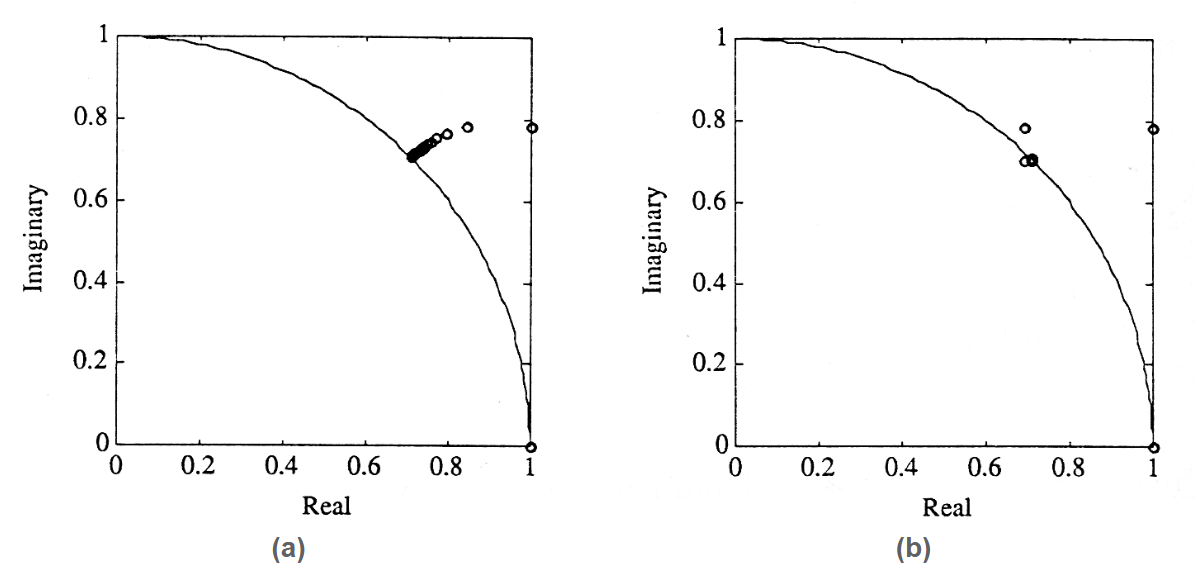
In this experiment, you will write a MATLAB program to evaluate the two functions \(f_n\) and \(S_n\) for twenty values of n:

1. \(f_n=(1+\frac {jθ} n)^n,\;n=1,2,...,20\) ; and
2. \(S_n=∑^n_{k=0}\frac {(jθ)^k} {k!},\;n=1,2,...,20k\)

Choose \(θ=π/4(=\mathrm{pi}/4)\). Use an implicit for loop to draw and plot a circle of radius 1. Then use an implicit for loop to compute and plot \(f_n\) and an explicit for loop to compute and plot \(S_n\) for n=1,2,...,100. You should observe plots like those illustrated in the Figure. Interpret them.

---