8.4: Summary

Graphical representations of power flow enable RF and microwave engineers to quickly ascertain circuit performance and arrive at qualitative design decisions. Humans are very good at processing graphical information and seeing patterns, anomalies, and the path from one point to another.

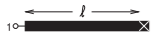
Figure \(\PageIndex{1}\): A \(50\:\Omega\) shorted gold microstrip line with width \(w = 500\:\mu\text{m}\), length \(\ell = 1\text{ cm}\) on a \(600\:\mu\text{m}\) thick alumina substrate with relative permittivity \(\varepsilon_{r} = 9.8\) and loss tangent \(\tan \delta = 0.001\).

The Smith chart is a richly annotated polar plot for representing reflection and transmission coefficients, and more generally, scattering parameters. The Smith chart representation of scattering parameter data aligns very well with the intuitive understanding of an RF designer. The experienced RF designer is intrinsically familiar with the Smith chart and prefers that circuit performance during design be represented on one. Representing something as simple as an extension of a line length to a two-port is quite complex if described using network parameters other than scattering parameters. However, with scattering parameters this extension results in a change of the angle of a scattering parameter, or on a Smith chart an arc. Scattering parameters relate directly to power flow. So from a Smith chart an experienced designer can ascertain the effect of circuit design on power flow, which then relates to signal-to-noise ratio and power gain.

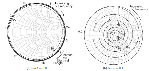
Figure \(\PageIndex{2}\): Smith chart plot of the reflection coefficient of the shorted \(1\text{ cm}\)-long microstrip line in Figure \(\PageIndex{1}\): (a) a low-loss substrate with \(\tan \delta = 0.001\); and (b) a high-loss substrate with \(\tan \delta = 0.1\). Frequencies are marked in gigahertz.

---