7.5: Iterative Mechatronic Control System Development and Validation Process- The V-Design Process

Example 7.3

For this example, we will essentially go through the mechatronic system design process shown in Figure 7.23, concentrated on Step 2. (The prototyping process in Step 3 varies significantly, depending on the type of mechatronic system.) Consider designing a three-wheel cart driving system with two active wheels. There are three design targets. First, for a maximum total vehicle mass of 6.5 kg with a certain payload, the vehicle should reach its peak speed of 0.6 m/s with a 5% settling time of 1.5 second. Second, the vehicle should be able to turn with differential steering. Third, the vehicle should be powered by a 12-volt battery.

For design Step 1, we need to generate a rough design for both the mechanical and electrical parts of this mechatronic system. Figure 7.24 shows a rough-designed drawing for the three-wheel cart. Due to the requirements of differential steering, both forward and backward driving, the three-wheel cart is designed with two front wheels powered by two geared DC motors. The differential steering can be realized by running the two front wheels in the opposite linear directions; operating both DC motors in the same linear direction leads to straight forward and backward movements. To increase the driving toque, a speed reduction gearbox is used in front of the DC-motor axis between the DC-motor axis and wheel axis. The 12-volt battery, microcontroller, certain sensors, and motor drive circuits are located inside the middle bay.

With Step 1 completed, we can now move to Step 2.1, developing a simplified system model so that certain system-related motor and sensor parameters can be determined through SiL simulations.

Assuming there is no wheel-slip on the road, the top plot of Figure 7.25 shows an equivalent vehicle model diagram. The two DC-motor circuits are merged into one. Assuming only forward or backward driving condition, the moment of inertia of the two driving wheels and motor rotors is lumped into a single moment of inertia \(J\). Total vehicle mass \(m\) includes all cart components. All frictions, including rolling resistance, are lumped into damping coefficient \(b_m\).

After this rough model is developed, we need to determine the model parameters so that a preliminary simulation can be conducted to validate the design feasibility. As noted in Section 2.4, the DC-motor inductance \(L_a\) can be assumed to be zero; it is normally much smaller than its resistance \(R_a\), which is assumed to be about 5 Ohms. Before determining preliminary motor coefficients \(K_τ\) and \(K_m\), we must determine the equivalent moment of inertia \(J+mR^2\). The wheel radius based on the rough design is about \(R=0.04\ m\). Assuming vehicle total mass to be \(7\ Kg\), the equivalent moment of inertia is \(mR^2=0.0112\ Kg\cdot m^2\). We will round that up to \(J_{total}=0.015\ Kg\cdot m^2\) to include the motor rotor and wheel moment of inertia. We will also assume that, at the target vehicle speed, the total friction torque will be around 6% of the motor peak torque.

Now we need to find the minimum \(K_τ\) and maximum \(K_m\) that defines the minimum requirements for the DC motors. Based upon the DC-motor torque curve defined in Section 5.2, the DC-motor output torque is a function of its motor speed as below, assuming that the inductance is zero (\(L_a=0)\).

\[ τ=\dfrac{{2K}_τ}{R_a}(v_a-K_mω) \label{7.6}\]

where the number \(2\) before the \(K_τ\) is due to the fact that there are two DC motors in the three-wheel cart. Assume that the target cart speed is reached at \(γ\) percent of the maximal motor speed \(ω_{no-load}\) with \(v_{a\_max}=12\ V\). As a result, we have

\[ ω_{no-load}=\dfrac{v_{v-max}}{K_{m-max}}\ =\dfrac{12\ (volt)}{K_{m-max}}=\dfrac{v_t}{γR}=\dfrac{1.2\ (m/s)}{0.04γ\ (m)}=\dfrac{30}{γ}\ (rad/s) \label{7.7}\]

where \(γ\) is a number between 0 and 1. Therefore,

\[ K_{m-max}=\dfrac{12\ (volt)}{30\ (rad/s)}γ=0.4γ\ (volt\times s/rad) \label{7.8}\]

To find \(K_{τ-min}\) (minimal \(K_τ\)), we are going to assume that the friction coefficient equals zero (\(b_m=0\)). The following dynamic equation can be obtained based upon the Newton’s law.

\[ J_{total}\dot{ω}=τ=\dfrac{{2K}_τ}{R_a}(v_a-K_mω) \label{7.9}\]

The following transfer function can be obtained after taking the Laplace transform of equation \ref{7.9} and simplifying it.

\[  \dfrac{Ω(s)}{V_a(s)}=\dfrac

Callstack:
    at (Bookshelves/Introductory_Engineering/Mechatronics:_Fundamentals_Design_Integration_and_Validation_(Zhu)/07:_Mechatronic_Control_Systems/7.05:_Iterative_Mechatronic_Control_System_Development_and_Validation_Process-_The_V-Design_Process), /content/body/section[2]/div/p[15]/span, line 1, column 2

With the design goal of 5% settling time of 1.5 second, we have the following.

\[  3T=1.5\ \left(second\right)\ \to \ K_{τ-min}=\dfrac{3}{1.5}\dfrac{R_aJ_{total}}{2K_{m-max}}=\dfrac{3\times 5\times 0.015}{1.5\times 2\times 0.4\times γ}=\dfrac{0.75}{4γ}\ (Nm/A) \label{7.11}\]

Next, we develop a model for a simulation study to confirm these selected parameters. The transfer function from \(E_a(s)\) to \(Ω(s)\) is shown below with \(K_{m-max}\) and \(K_{τ-min}\) substituted, assuming \(L_a\approx 0\) and \(b_m\approx 0\).

\[ \ G\left(s\right)=\dfrac{Ω\left(s\right)}{E_a\left(s\right)}=\dfrac{2K_τ}{R_a\left(Js+b_m\right)+2K_τK_m}=\dfrac{1.5/γ}{0.075s+0.15}=\dfrac{10/γ}{0.5s+1}=\dfrac{K}{Ts+1} \label{7.12}\]

As a result, the time constant is about 0.5 second and the 5% settling time \(t_s\) is about \(3T=1.5\) seconds with satisfactory performance.

In the next step (Step 2.2) we select the speed sensor and DC-motor actuator so that we can develop a complex mathematical (nonlinear) model. Assuming that there is no slip between tire and road, we need to select DC motors and associated motor speed sensors for these two motors. For the speed sensor, the hall-effect sensor is a good choice due to its high signal-to-noise ratio at high speed. However, the hall-effect sensor signal-to-noise ratio reduces as the axis speed goes down for a given sample rate. As the sample period reduces, the number of pulses available to be counted during that period also reduces. Therefore, selecting a hall effect sensor depends on the control system sample rate and minimal motor shaft speed. The control sample frequency of the three-wheel cart is about \(f_h=1/(2πT)\ Hz\). We can assume that the highest control loop sample frequency of 50 Hz. It is desirable to have at least 10 pulses at the vehicle speed of \(0.1\ m/s\). We can calculate the corresponding wheel speed as follows.

\[  ω_{wheel}\left(0.05\right)=\dfrac{v_{vehicle}}{R_{wheel}}=\dfrac{0.1}{0.04}=2.5\ (rad/s) \label{7.13}\]

With a sample period of \(T_s=0.02\) second, the wheel rotation angle \(θ_{wheel}\) over each sample period is \(θ_{wheel}=0.02\times 2.5=0.05\) (rad). Therefore, to have at least 10 pulses, we can calculate the number of pulses per wheel rotation can as below.

\[  n_{p-req}=\dfrac{2π}{θ_{wheel}}\times 10=1257 \label{7.14}\]

The selected motor and encoder set is model B09MFT3VT7 (or JGB37-520-12V-333RPM) with DC-motor parameters \(K_τ=0.00767\ (Nm/A)\) and \(K_m=0.81\ (V\times s/rad)\) that are not satisfactory for the required \(K_{τ-min}=0.15\ (Nm/A)\) and \(K_{m-max}=0.1\ (Vs/rad)\) with any \(0<γ<1\). As a result, we select a gearbox with a speed reduction ratio of \(30:1\) at the motor driving shaft to move both parameters into the feasible ranges as below with \(γ=0.5\).

\[  K_{τ-g}=30K_τ=0.23>K_{τ-min}=0.2, K_{m-g}=\dfrac{K_m}{30}=0.027<K_{m-max}=0.375\ \label{7.15}\]

For the encoder speed sensor, the selected available hall-effect sensor is an eleven-pulse per revolution one. In this case, one revolution of the gear-box output shaft leads to 330 (\(30\times 11\)) pulses, which is below the required 1257. A gearbox with ratio of 1:4 from motor to encoder shaft is employed to make

\[ n_p=11\times 4\times 30=1320\ >\ n_{p-req}=1257\ (\ of\ pulse\ per\ revolution) \label{7.16}\]

Now we develop a detailed mathematical model for simulation validation (Step 2.3). We will begin by developing the three-wheel cart equations of motion (EOMs). Figure 7.26 shows the cart free body diagram.

Assuming that there is no slip between wheel and ground, the following EOMs can be developed based upon Newton’s law, with \(v=\dot{x}\) and \(ω=\dot{θ}\).

\[ \ m\dot{v}+b_vv=f_L+f_R, J_v\dot{ω}+b_θω=\left(f_L-f_R\right)R_v\ \label{7.17}\]

where \(m=6.5\) (\(Kg\)) and \(J_v\approx 0.02\) (\(Kg{\times m}^2\)) are cart mass and moment of inertia around the center of mass, respectively; \(b_v\approx 0.1\) (\(Ns/m\)) and \(b_θ\approx 0.01\) (\(Nms/rad\)) are the cart mass and moment of inertia around center of mass, respectively; and \({R_v, f}_L\), and \(f_R\) are the half distance between the two driving wheels, left and right wheel driving forces marked on Figure 7.26, respectively. As a result, the following transfer functions can be derived for the three-wheel cart.

\[V\left(s\right)=\dfrac{1}{ms+b_v}\left(F_L\left(s\right)+F_R\left(s\right)\right), Ω\left(s\right)=\dfrac{1}{J_vs+b_θ}\left(F_L(s)-F_R(s)\right)R_v\ \label{7.18}\]

where \(V\left(s\right)\) and \(Ω\left(s\right)\) are Laplace transforms of \(v(t)\) and \(\dot{θ}(t)\), respectively, and \(F_L\left(s\right)\) and \(F_R\left(s\right)\) are Laplace transforms of \(f_L\) and \(f_R\). After the three-wheel cart linear movement speed \(v(t)\) and its rotational movement \(\dot{θ}(t)\) around the vertical axis are calculated, the three-wheel cart linear speed at each wheel can be calculated as below.

\[\ v_L\left(t\right)=v\left(t\right)+R_v\dot{θ}\left(t\right), v_R\left(t\right)=v\left(t\right)-R_v\dot{θ}(t)\ \label{7.19}\]

where \(R_v=0.18415\ (m)\) is the half distance of the two front driving wheels (see Figure 7.26), and \(v_L\left(t\right)\) and \(v_R\left(t\right)\) are the three-wheel cart linear speeds at the left and right wheels. Now the corresponding wheel speed can be calculated as below.

\[{\dot{θ}}_L\left(t\right)=ω_L(t)=\dfrac{v_L\left(t\right)}{R_w}\dot{θ}\left(t\right), {\dot{θ}}_R\left(t\right)=ω_R(t)=\dfrac{v_R\left(t\right)}{R_w}\ \label{7.20}\]

where \(R_w=0.0381\ (m)\) is the radius for both driving wheels, \({\dot{θ}}_L\left(t\right)=ω_L(t)\) and \({\dot{θ}}_R\left(t\right)=ω_R(t)\) are the left and right driving wheel angular speeds, respectively.

Once all the mathematical equations have been derived for the detailed model, we can use Simulink to develop a detailed simulation model. See Figure 7.27, where the model includes both DC-motor dynamics (labeled “Motor dynamics”). Here, \(R_a=5.0\ (Ω\mathrm{)}\), \(L_a=2\ (mH)\), \(K_τ=0.23\ (Nm/A)\), and \(K_m=0.027\ \left(Vs/rad\right)\). Note that the torque and back-EMF coefficients used are these equivalent ones for the geared output shaft.

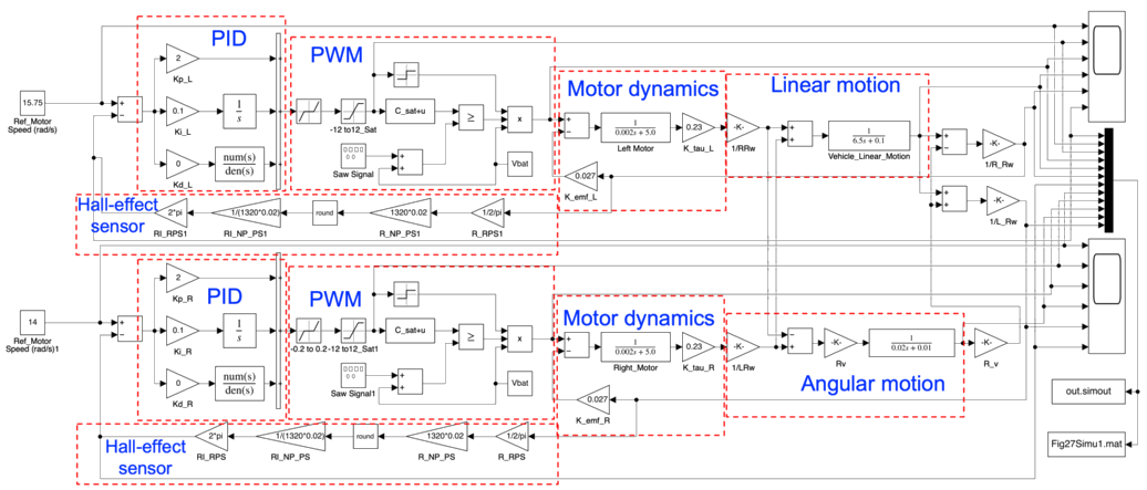
For the three-wheel cart, the vehicle dynamics is modeled using equation \ref{7.18} for both linear and rotational motions; see the red-dashed line blocks marked “Linear motion” and “Angular motion,” respectively. We can use equation \ref{7.18} to calculate the overall three-wheel cart speed \(v(t)\) and angular speed \(ω(t)\); equation \ref{7.19} to calculate the linear cart speed signals \(v_L\left(t\right)\) and \(v_R\left(t\right)\) at both driving wheels; and equation \ref{7.20} to calculate both wheel speed signals \(ω_L(t)\) and \(ω_R(t)\). See the right side of the “Linear motion” and “Angular motion” blocks in the Simulink model.

Both DC motors will be controlled by PWM signals (see Chapter 5). Therefore, we need to simulate the effect of PWM control signals in the detailed model, especially for the effect of the selected PWM frequency. Figure 7.27 shows two red-dashed blocks marked as “PWM” for both DC-motor models. Within each of these blocks, the PWM driving signal of the DC motor is generated using a 12-volt saw wave generated by Simulink signal generation block, where its peak is 12 volts and its bottom is –12 volts. The saw wave signal is then shifted by a 12-volt battery signal to make it a saw wave signal with its peak equal to 24 volts and bottom 0 volt. To generate a PWM signal with its duty-cycle proportional to the saturated control signal, we shift the saturated control signal with a range of \(\pm C_{sat}\) by \(C_{sat}\). The shifted control then has a range between 0 and \({2C}_{sat}\) volt. If \(C_{sat}=12\) volts, the shifted control signal has a range between 0 and 24 volts, the same as that of the shifted saw wave. The shifted control signal is compared with the shifted saw wave. If the control signal is greater than or equal to the saw wave signal, the logical output is 1. Otherwise, it’s zero. Finally, we can obtain the PWM signal output by multiplying the battery voltage by the logical output.

To simulate digital angular speed of the hall-effect sensor, we convert the continuous-time wheel speed signal to the number of pulses for a given sample period \(T_s=0.02\ (s)\). Divide by \(2π\), then multiply the number of pulses per motor revolution (1320) and sample period (0.02 s). Then round off the real number to the closest integer. Next, apply the reverse process, dividing \(1320\times T_s\) and multiplying by \(2π\). Through this process, we simulate the roundoff effect of the digital hall-effect sensor. Figure 7.27 has two red-dashed line blocks, named Hall-effect sensor, for roundoff operations for the two encoders mounted on the DC motors. Modeling the roundoff error of the hall-effect sensor shows the effect of the hall-effect sensors.

The last two red-dashed line blocks in Figure 7.27, named PID, are the two PID controllers. They take the DC-motor speed signals measured by hall-effect sensors as feedback signals; the error signal was calculated by subtracting the measured DC-motor speed signal from the given reference motor speed. Due to slow cart dynamics, the derivative gains of both PID controllers are set to zero; the proportional and integral gains are set to 2 and 0.1 respectively for both controllers.

The detailed mathematical model developed above can be further improved by adding sample and hold mechanism so that a digital controller can be simulated. With the detailed model now developed, we can move to Step 2.5 for simulation studies to evaluate the system’s performance. In practice, we should develop a test plan to validate the design. This example conducts two simulation studies: linear acceleration motion and angular acceleration motion. Figure 7.28 shows the linear forward motion simulation results. The reference wheel speed for both left and right are \(\mathrm{15.75\ (}rad\mathrm{/}s\mathrm{)}\). With wheel radius \(R_w\mathrm{=0.0381\ (}m\mathrm{)}\), the target vehicle linear speed under these wheel speeds is

\[v=\dfrac{(ω_R+ω_L)R_w}{2}=\dfrac{(15.75+15.75)\times 0.0381}{2}=0.6\ (m/s) \label{7.21}\]

Figure 7.28 has five plots. The top two plots (red lines) show the continuous-time saturated PID control outputs for both left and right motor speed control. The blue pulses are the PWM drive signals for both left and right motors. In this simulation, the continuous-time control signals are saturated at 6 volts to simulate a situation with low-voltage power supply. We can see that when the control voltage is saturated at 6 volts, the PWM drive signals are at 50% duty-cycle. As the magnitude of continuous-time control signal reduces, the corresponding PWM signal duty-cycle also reduces. After 0.3 second, the vehicle reaches its steady-state; the duty-cycle of the PWM signal reduces to a level that maintains the vehicle at its target speed of 0.6 (m/s). Also, the control signal is saturated at the beginning, leading to a nonlinear simulation.

The third and fourth plots show the reference and simulated left and right wheel speed signals. The blue lines are the reference wheel speed signals for the left and right wheels. The red lines represent the simulated speeds of the left and right wheels. The two thin orange lines are the simulated speeds of the left and right wheels measured by the hall-effect sensors. We can see that the speed signals measured by hall-effect sensors fluctuate around the simulated speed signals due to a finite number of pulses. It takes about 0.3 second for both wheels to reach their steady-state angular speeds of \(15.75\ rad/s\). Both wheels accelerate synchronously to reach the steady state speed. Recall that the simulation was conducted assuming no wheel slip; with slip, the acceleration will be slower.

The bottom graph of Figure 7.28 shows both the simulated linear cart speed and angular cart rotation rate (speed). The cart speed reaches \(0.6\ m/s\) within \(0.3\) second, which is less than the required \(5\%\) settling time of \(1.5\) seconds. As a result, both design goals of maximum cart speed of \(0.6\ m/s\) and \(5\%\) settling time of \(1.5\) second are satisfied. Because both motor speeds are synchronous, the angular cart speed is zero.

Figure 7.29 shows the simulation results with different reference wheel speeds and five subplots. (The left wheel is 14 rad/s and the right wheel is 15.75 rad/s). The top two subplots show the continuous-time saturated PID control outputs (red lines) and PWM drive signals (blue lines) for both left and right motors. In this simulation, the continuous-time control signals are also saturated at 6 volts. When the control voltage is saturated at 6 volts, the PWM drive signals are at 50% duty-cycle. As the magnitude of continuous-time control signal reduces, the corresponding PWM signal duty-cycle also reduces. After \(0.3\) second, the vehicle reaches its steady state, and the duty cycle of the PWM signal reduces. Different from Figure 7.28 due to different reference wheel speeds for the two wheels, the continuous-time control signal of the left motor decays earlier than the right one due to its reference speed being slower than the right one.

The third and fourth subplots of Figure 7.29 show the reference and simulated wheel speed signals, with blue lines for reference wheel speed signals and two red lines for simulated wheel speeds. Two thin orange lines present the simulated wheel speeds measured by the hall-effect (HE) sensors with digitization errors. Due to the control saturation, the two wheels accelerate at the same rate. However, after about 0.2 second, the left wheel acceleration becomes smaller than that of the right one due to its lower reference speed. Similarly, it takes about 0.3 second for both wheels to reach their steady-state angular speeds of \(15.75\) and \(14\) rad/s.

The bottom subplot of Figure 7.29 also shows both simulated linear cart speed and angular cart rotation rate (speed). The cart speed reaches \(0.5647\ m/s\) within 0.3 second. The angular speed of the cart starts at zero due to synchronous acceleration of both wheels until around 0.2 seconds. It then gradually reduces down to \(-0.1667\ rad/s\) with certain oscillations due to the sparse PWM pulse at the steady state. This simulation results suggest using high PWM frequency.

In Step 2.6, we decide if the design needs to be optimized. If so, the process will go back to Step 2.1 (Rough mathematical model) to start a new design iteration. If the design is satisfactory, we move to Step 3.

In Step 3.1, we conduct an HiL simulation study. Our purpose is to select a proper microcontroller. We also want to select the associated drives (power amplifiers) for the selected actuators and the associated input channels for the selected sensors (Step 2.2). There are various levels of HiL simulation studies we can develop. They have different purposes, from validating the selected microcontroller and associated electronic systems to the entire mechatronic system. The HiL system is widely used due to its simplicity.

Figure 7.30 shows an HiL system developed to validate the microcontroller capability and associated electronic components. Here, the Arduino MKR 1000 Wi-Fi microcontroller and an Arduino MKR motor carrier board are used. The system also includes two DC motor and hall-effect sensor assemblies (see the right-side of Figure 7.30). Now with this HiL system in place, we can develop the associated two-motor speed control software in Simulink by doubling the motor speed controller shown in Figure 7.21. By running the HiL simulations, we can validate the feasibility of using the Arduino MKR 1000 Wi-Fi and its motor carrier board.

Next, in Step 3.2, we deploy all the selected hardware to the designed prototype three-wheel cart shown in Figure 7.24. Then we conduct validation tests on the prototype similar to these described in Step 2.5. If the prototype’s performance is not satisfactory, we improve the mechatronic system until the performance is satisfactory. The actual deployment of the three-wheel cart deployment can be found in Chapter 9.

After meeting the prototype’s performances, the next step (Step 3.3) is to optimize the prototype system for massive production. For example, the current three-wheel cart speed settling time is about 0.3 second with a requirement of 1.5 second. Therefore, to reduce system cost, we would look for a smaller motor with less torque output than the already-selected one. With any modification, we conduct a design iteration. Because the system model and simulation platform have been mostly developed, the next iteration is fairly fast; we can obtain the final prototype results.