4.4: Analog and Digital Filter Design

Learning Objectives

After completing this section, you will be able to:

1. Provide concepts of analog and digital filtering.
2. Describe low-pass, high-pass, band-pass, and notch (band-kill) filtering concepts.
3. Design low-pass, high-pass, band-pass, and notch filters (analog and digital).
4. Provide working principles of analog filter realization circuits.

This section discusses the signal conditioning of both analog and digital signals to get rid of unwanted signal components such as sensor noise. We will first address the widely used low- and high-pass filtering concepts and the associated design methodologies, along with their realizations. We will then discuss the band-pass and band-kill (notch) filters based on low- and high-pass filters.

In general, the filter design is conducted in the frequency domain. Let \(U\left(s\right)\) be the Laplace transform of the signal to be filtered, \(Y\left(s\right)\) the Laplace transform of filtered signal, and \(F\left(s\right)\) the continuous-time filter transfer function. Then,

\[ Y\left(s\right)=F\left(s\right)U(s) \label{4.57}\]

Similarly, let \(U\left(z\right)\) be the \(z\)-transform of the signal to be filtered, \(Y\left(z\right)\) be the \(z\)-transform of filtered signal, and \(F\left(z\right)\) the discrete-time filter transfer function. Then,

\[Y\left(z\right)=F\left(z\right)U\left(z\right)\ \label{4.58}\]

First, let’s consider the case of low-pass filtering. Ideally, for a given cutoff frequency \(ω_c\), the low-pass filter allows the signal frequency component below \(ω_c\) to pass while denying the signal frequency component above \(ω_c\); see the left plot of Figure 4.28. That is, below the cutoff frequency, \(ω\mathrm{<}ω_{\mathrm{c}}\), \(\left|F\left(jω\right)\right|\mathrm{=1}\), allow the low frequency signal to pass. Beyond the cutoff frequency, \(ω\mathrm{>}ω_{\mathrm{c}}\), \(\left|F\left(jω\right)\right|\mathrm{=0}\), preventing the high frequency signal from passing.

If, for a continuous-time low-pass filter transfer function, we want to ensure that the magnitude of the frequency response goes to zero as the frequency increases to infinity, then the order of the denominator’s polynomial must always be higher than the numerator’s. In other words, there are more poles than zeros for a low-pass filter transfer function. On the other hand, there is also no pole nor zero at the origin of the complex plan. Therefore, the low frequency response magnitude has non-zero finite value. The right plot of Figure 4.28 illustrates the result of the signal defined in equation \ref{4.50}, filtered by the ideal low-pass filter with \(ω_c=2.03\) rad/s. We can see that the frequency response was cut off after the cutoff frequency \(ω_c=2.03\) rad/s.

However, the ideal low-pass filter is not realizable using a rational-proper transfer function that has finite order with numerator’s polynomial order less than or equal to that of denominator’s polynomial. The typical first order low-pass filter transfer function \(F_{L1}\left(s\right)\) with unit gain is shown below.

\[F_{L1}\left(s\right)=\dfrac{ω_c}{s+ω_c} \label{4.59}\]

The typical second order low-pass filter transfer function \(F_{L2}\left(s\right)\) with unit gain is presented below.

\[F_{L2}\left(s\right)={\left(\dfrac{ω_c}{s+ω_c}\right)}^2=\dfrac{ω^2_c}{s^2+2ω_cs+ω^2_c} \label{4.60}\]

Note that the unit gain of a transfer function can be confirmed by setting \(s\) to zero for both first and second order filter transfer functions. We can see the frequency responses of both first and second order low-pass filters in the top plot of Figure 4.29. Comparing these responses to the ideal low-pass filter characteristics in Figure 4.28, we can see that neither the first or second order low-pass filters from equations \ref{4.59} and \ref{4.60} kill the frequency response beyond the cutoff frequency \(ω_c\). Instead, they only reduce the gain beyond cutoff frequency \(ω_c\). Here, the first order low-pass filter reduces signal magnitude by 20 dB every 10 times frequency after the cutoff frequency. In addition, the second order low-pass filter reduces signal magnitude by 40 dB every 10 times frequency after the cutoff frequency.

Working from the bottom plot of Figure 4.28, for the frequency response presented in Figure 4.29 (blue line), the first order low-pass filtered frequency response is shown by the dashed-red line. The second order response is shown by the green dash-dot line. As the low-pass filter order increases, the decrement rate of frequency response magnitude after the cutoff frequency increases. Note that the high-order low-pass filter can also be implemented in the form below.

\[F_{Ln}\left(s\right)={\left(\dfrac{ω_c}{s+ω_c}\right)}^n \label{4.61}\]

where \(n>0\) (integer) is the order of the low-pass filter. Advanced high order low-pass filter design will be addressed in Section 4.7.

Analog filters can be implemented using analog circuits. Figure 4.30 shows two circuits that can be used to realize the first order low-pass analog filter based upon an RC (resistor and capacitor) circuit. Its first order transfer function can be derived utilizing the circuit modeling knowledge from Chapter 2. Note that high-order analog low-pass filters can also be realized by repeating the circuit shown in the right side of Figure 4.30.

The left circuit of Figure 4.30 is called an RC circuit for low-pass filter. The right circuit provides the same transfer function with an additional isolation circuit to make the low-pass circuit output impedance equal to zero. In that way, the filter characteristics will not be altered after it is connected to the other circuit. Utilizing the knowledge learned from Chapter 2, the transfer function of this circuit can be derived below.

\[F_{L1}\left(s\right)=\dfrac{V_{out}(s)}{V_{in}(s)}=\dfrac{1}{sRC+1}=\dfrac{1/RC}{s+1/RC} \label{4.62}\]

As a result, the cutoff frequency of the low-pass filter in Figure 4.30 is \(ω_c=1/RC\). For a given cutoff frequency, there exist infinite combinations of resistor and capacitor values, where the resistor and capacitor values need to be selected properly for feasible implementation.

Example 4.11

For the second order low-pass filter transfer function defined in equation \ref{4.60}, design an electronic circuit and find resistor and capacitor values to have a cutoff frequency of \(ω_c=10\) rad/s. Note that the second order low-pass filter can be realized by repeating the first order circuit as below.

Due to the isolation circuit in the middle, the transfer function of the circuit in Figure 4.31 is shown below.

\[ F_{L2}\left(s\right)=\dfrac{V_{out}(s)}{V_{in}(s)}={\left(\dfrac{1/RC}{s+1/RC}\right)}^2 \label{4.63}\]

Because the cutoff frequency is \(ω_c=1/RC\), to make \(ω_c=10\), let \(R=1\) \(kΩ\) and we can calculate the capacitor value as below.

\[ C=\dfrac{1}{Rω_c}=\dfrac{1}{{10}^3\times 10}=100\ μF \label{4.64}\]

Next, we will consider the case of high-pass filtering. For a given cutoff frequency \(ω_c\), the high-pass filter ideally allows the signal frequency component beyond \(ω_c\) to pass while denying the signal frequency component below \(ω_c\); see the left plot of Figure 4.32. That is, below the cutoff frequency, \(ω\mathrm{<}ω_{\mathrm{c}}\), \(\left|F\left(jω\right)\right|\mathrm{=0}\), it prevents low frequency signals passing and, beyond the cutoff frequency, \(ω\mathrm{>}ω_{\mathrm{c}}\), \(\left|F\left(jω\right)\right|\mathrm{=1}\), it allows high frequency signals to pass.

Assume we want to ensure that the magnitude of the frequency response goes to one at the frequency beyond \(ω_{\mathrm{c}}\). In this case, for the continuous-time filter transfer function, the denominator’s polynomial order should be equal to that of numerator. In other words, the numbers of poles and zeros need to be the same for a high-pass filter transfer function. On the other hand, at least one zero is needed at the origin of the complex plan to make it possible to have zero value at a frequency equal to zero. The right plot of Figure 4.32 illustrates the result of the signal defined in equation \ref{4.50} filtered by an ideal high-pass filter with \(ω_c=2.03\) rad/s. We can see that the frequency response was cut off before the cutoff frequency \(ω_c=2.03\) rad/s.

From a practical perspective, the ideal high-pass filter is not realizable using a rational-proper transfer function with finite orders of both numerator and denominator’s polynomials. The typical first order high-pass filter transfer function \(F_{H1}\left(s\right)\) with unit gain is shown below.

\[F_{H1}\left(s\right)=\dfrac{s}{s+ω_c} \label{4.65}\]

In turn, the typical second order high-pass filter transfer function \(F_{H2}\left(s\right)\) with unit gain is shown below.

\[F_{H2}\left(s\right)={\left(\dfrac{s}{s+ω_c}\right)}^2=\dfrac{s^2}{s^2+2ω_cs+ω^2_c} \label{4.66}\]

The unit gain at frequencies higher than the cutoff frequency \(ω_c\) can be confirmed by letting \(s\) go to infinity for both first and second order high-pass filter transfer functions. The frequency responses of these filters can be found in the top plot of Figure 4.33. Compared with the ideal high-pass filter characteristics in Figure 4.32, we can see that, instead of killing the frequency response below the cutoff frequency, both first and second order low-pass filters from equations \ref{4.65} and \ref{4.66} reduce the signal magnitude. The first order high-pass filter reduces signal magnitude by 20 dB every 10-time frequency below the cutoff frequency (20 dB increment per 10-time frequency). The second order high-pass filter reduces signal magnitude by 40 dB every 10 times frequency before the cutoff frequency (40 dB increment per 10-time frequency). In addition, compared to the low-pass filter case, the characteristics of the high-pass filter are symmetric to the low-pass filter around the vertical axis at the cutoff frequency.

For the frequency response presented in Figure 4.32 (blue line), the first order high-pass filtered frequency response is shown in the dashed-red line in the bottom plot of Figure 4.33. The second order high-pass filtered frequency response is represented by the green dash-dot line. We can see that as the high-pass filter order increases, the frequency response magnitude decreases before the cutoff frequency. Also, note that high-order high-pass filters can be implemented in the form below.

\[F_{Hn}\left(s\right)={\left(\dfrac{s}{s+ω_c}\right)}^n \label{4.67}\]

where \(n>0\) (integer) is the order of the high-pass filter. Advanced high-order high-pass filter design will be addressed in Section 4,7. We will now again address how to implement the analog high-pass filters using analog CR (capacitor and resistor) circuits based on the circuit modeling knowledge from Chapter 2. High-order analog high-pass filters can also be realized based on this circuit. The first order high-pass filter can be realized using the circuit shown in Figure 4.34. Here, the left circuit is a CR circuit for a high-pass filter; the right circuit provides the same transfer function with an additional isolation circuit to make the high-pass circuit output impedance equal to zero. Utilizing the knowledge learned from Chapter 2, the transfer function of the circuit in Figure 4.34 can be derived below.

\[F_{H1}\left(s\right)=\dfrac{V_{out}(s)}{V_{in}(s)}=\dfrac{sRC}{sRC+1}=\dfrac{s}{s+1/RC} \label{4.68}\]

As a result, the cutoff frequency of the high-pass filter in Figure 4.34 is \(ω_{\mathrm{c}}\mathrm{=}1/RC\). Similar to the case of the low-pass filter, for a given cutoff frequency, infinite combinations of resistor and capacitor values exist.

Example 4.12

For the second order high-pass filter transfer function defined in equation \ref{4.66}, design an electronic circuit. Then find resistor and capacitor values to have a cutoff frequency of \(ω_c={10}^4\) rad/s. Note that the second order high-pass filter can be realized by repeating the first order circuit from Figure 4.34.

Given the isolation circuit in the middle, the transfer function of the circuit in Figure 4.35 is shown below.

\[ F_{H2}\left(s\right)=\dfrac{V_{out}(s)}{V_{in}(s)}={\left(\dfrac{s}{s+1/RC}\right)}^2 \label{4.69}\]

Because the cutoff frequency is \(ω_c=1/RC\), to make \(ω_c={10}^4\), let \(R=1\) \(kΩ\). we can then calculate the capacitor value as below.

\[ C=\dfrac{1}{Rω_c}=\dfrac{1}{{10}^3\times {10}^4}=0.1\ μF \label{4.70}\]

Next, let’s consider the case of band-pass filtering. Ideally, for a pair of given cutoff frequencies \(ω_{c_1}\) and \(ω_{c_2}\), the band-pass filter allows the signal frequency component between \(ω_{c_1}\) and \(ω_{c_2}\) to pass while denying the signal frequency component below \(ω_{c_1}\) and beyond \(ω_{c_2}\); see the left plot of Figure 4.36. That is, below the first cutoff frequency, \(ω\mathrm{<}ω_{c_1}\), and beyond the second cutoff frequency, \(ω\mathrm{>}ω_{c_2}\), \(\left|F\left(jω\right)\right|\mathrm{=0}\), preventing low and high frequency signal components from passing. At the middle frequency \(ω_{c_1}<ω\mathrm{<}ω_{c_2}\), \(\left|F\left(jω\right)\right|\mathrm{=1}\), allowing middle frequency signal components to pass.

In order to ensure that the magnitude of the frequency response goes to one at the frequency between \(ω_{c_1}\) and \(ω_{c_2}\), the denominator’s polynomial order should be higher than the numerator’s. In other words, the number of poles should be greater than the number of zeros for a band-pass filter transfer function. On the other hand, there is also at least one zero at the origin of the complex plan to make it possible to have zero value at a frequency equal to zero. The right plot of Figure 4.36 illustrates the result of the signal defined in equation \ref{4.71} filtered by the ideal band-pass filter with \(ω_{c_1}=1.68\) and \(ω_{c_2}=6.91\) rad/s. We can see that the frequency response was cut off before the first cutoff frequency \(ω_{c_1}=1.68\) rad/s and after the second cutoff frequency \(ω_{c_2}=6.91\) rad/s.

\[U\left(s\right)=\dfrac{1}{s^2+1}+0.5\dfrac{10}{s^2+100}+\dfrac{3}{s^2+9}=\dfrac{9s^4+462s^2+1245}{s^6+110s^4+1009s^2+900} \label{4.71}\]

The ideal band-pass filter can be designed based on the ideal low- and high-pass filters with low-pass filter cutoff frequency \(ω_{c_2}\) greater than the high-pass filter cutoff frequency \(ω_{c_1}\). Figure 4.37 illustrates using serially connected low- and high-pass filters to form a band-pass filter. Therefore, the band-pass filter can be formed based on the techniques discussed earlier in this section for both low- and high-pass filters.

Again, the ideal band-pass filter is not realizable using a rational-proper transfer function with finite orders of both numerator and denominator’s polynomials. The typical first order band-pass filter transfer function \(F_{B1}\left(s\right)\) with unit gain is shown below by serially connecting the low- and high-pass filters.

\[F_{B1}\left(s\right)=F_{L1}\left(s\right)F_{H1}\left(s\right)=\dfrac{s}{s+ω_{c_1}}\dfrac{ω_{c_2}}{s+ω_{c_2}},\ ω_{c_2}>ω_{c_1} \label{4.72}\]

The typical second order band-pass filter transfer function \(F_{B2}\left(s\right)\) with unit gain is shown below.

\[F_{B2}\left(s\right)={\left(\dfrac{s}{s+ω_{c_1}}\dfrac{ω_{c_2}}{s+ω_{c_2}}\right)}^2=\left(\dfrac{s^2}{s^2+2ω_{c_1}s+ω^2_{c_1}}\right)\left(\dfrac{ω^2_{c_2}}{s^2+2ω_{c_2}s+ω^2_{c_2}}\right) \label{4.73}\]

The frequency responses of both first and second order band-pass filters with \(ω_{c_1}=1.68\) and \(ω_{c_2}=6.91\) rad/s can be found on the top plot of Figure 4.38. Compared with the ideal band-pass filter characteristics from Figure 4.36, we can see that, instead of killing the frequency response below the cutoff frequency \(ω_{c_1}=1.68\) and beyond frequency \(ω_{c_2}=6.91\), both first and second order band-pass filters from equations \ref{4.72} and \ref{4.73} reduce the magnitude before the first cutoff frequency \(ω_{c_1}\). After the second cutoff frequency \(ω_{c_2}\), the first order band-pass filter reduces signal magnitude by 20 dB every 10 times frequency below the cutoff frequency \(ω_{c_1}\) and beyond cutoff frequency \(ω_{c_2}\) (20 dB increment per 10-time frequency). The second order band-pass filter reduces signal magnitude by 40 dB every 10 times frequency before the cutoff frequency \(ω_{c_1}\) and beyond cutoff frequency \(ω_{c_2}\) (40 dB increment per 10-time frequency).

In addition, the characteristics of the band-pass filter have properties similar to high-pass filters below cutoff frequency \(ω_{c_1}\) and have properties similar to low-pass filters beyond cutoff frequency \(ω_{c_2}\). In the bottom plot of Figure 4.38, the original frequency response is shown by the blue-line, the first order band-pass filtered frequency response is represented by the dashed-red line, and the second order high-pass filtered frequency response is shown in the green dash-dot line. We can see that as the band-pass filter order increases, the decrement rate of frequency response magnitude increases before the cutoff frequency \(ω_{c_1}\) and beyond the cutoff frequency \(ω_{c_2}\).

Also, the high-order band-pass filter can be implemented in the form below.

\[F_{Bn}\left(s\right)={\left(\dfrac{s}{s+ω_{c_1}}\right)}^n{\left(\dfrac{ω_{c_2}}{s+ω_{c_2}}\right)}^n \label{4.74}\]

where \(n>0\) (integer) is the order of the band-pass filter. Advanced high-order band-pass filter design will be addressed in Section 4.7.

Now, we will address implementing the analog band-pass filters using analog resistor and capacitor (RC) circuits based on the circuit modeling knowledge from Chapter 2. Note that high-order analog band-pass filters can also be realized using similar circuits.

The first order band-pass filter can be realized using the circuit shown in Figure 4.39. Here, the high-pass filter is isolated from the second low-pass filter, where the order of RC circuits for both high-pass and low-pass filters can be switched. That is, we can have the high-pass filter on the left and the low-pass filter on the right, to have the same band-pass transfer function. Utilizing what we learned in Chapter 2, the transfer function of the above circuit can be derived and listed below.

\[F_{B1}\left(s\right)=\dfrac{V_{out}(s)}{V_{in}(s)}=\left(\dfrac{sR_HC_H}{sR_HC_H+1}\right)\left(\dfrac{R_LC_L}{s+R_LC_L}\right) \label{4.75}\]

As a result, the cutoff frequencies of the band-pass filter in Figure 4.39 are \(ω_{c_1}=1/R_HC_H\) and \(ω_{c_2}=1/R_LC_L\ \)with \(R_HC_H\) greater than \(R_LC_L\). Similar to the case of low- and high-pass filters, for any given cutoff frequency, infinite combinations of resistor and capacitor values exist. We can realize the second order band-pass filter in a similar manner by replacing the first order low- and high-pass filters with the second order ones, respectively.

Example 4.13

For the first order band-pass filter circuit defined in Figure 4.39 with its transfer function defined in equation \ref{4.75}, find resistor and capacitor values to have cutoff frequencies \(ω_{c_1}=1.68\) and \(ω_{c_2}=6.91\) rad/s (used in the simulations in Figure 4.38) for given resistor values \(R_H=R_L=100\ kΩ\).

Because the low cutoff frequency is \(ω_{c_1}=1/R_HC_H=1.68\) rad/s, to make \(ω_{c_1}=1.68\), we can calculate the capacitor value \(C_H\) as below.

\[ C_H=\dfrac{1}{R_Hω_{c_1}}=\dfrac{1}{{10}^5\times 1.68}=5.952\ μF \label{4.76}\]

For the second cutoff frequency of \(ω_{c_2}=1/R_LC_L=6.91\) rad/s, to make \(ω_{c_2}=6.91\), we can calculate the capacitor value \(C_L\) as below.

\[ C_L=\dfrac{1}{R_Lω_2}=\dfrac{1}{{10}^5\times 6.91}=1.447\ μF \label{4.77}\]

Next, we will consider the case of band-kill (notch) filtering. For a pair of given cutoff frequencies \(ω_{c_1}\) and \(ω_{c_2}\), the band-kill filter ideally allows the signal frequency component below \(ω_{c_1}\) and beyond \(ω_{c_2}\) to pass while denying the signal frequency component between \(ω_{c_1}\) and \(ω_{c_2}\); see the left plot of Figure 4.40. That is, at frequencies \(ω\mathrm{<}ω_{c_1}\) and \(ω\mathrm{>}ω_{c_2}\), \(\left|F\left(jω\right)\right|\mathrm{=1}\), allowing low and high frequency signal component to pass. At the middle frequency \(ω_{c_1}<ω\mathrm{<}ω_{c_2}\), \(\left|F\left(jω\right)\right|\mathrm{=0}\), denying high frequency signal component to go through.

In order to ensure that the magnitude of the frequency response goes to one as frequency goes to infinity, the order of denominator’s polynomial should equal the numerator’s. In other words, the number of poles should be equal to that of zeros for a band-kill filter transfer function. On the other hand, there is no zero (nor pole) at the origin of the complex plan to have finite non-zero magnitude at frequency equal to zero (on infinity). The right plot of Figure 4.40 illustrates the result of the signal defined in equation \ref{4.71} filtered by the ideal band-kill filter with \(ω_{c_1}=1.68\) and \(ω_{c_2}=6.91\) rad/s. We can see that the frequency response was cut off between the first cutoff frequency \(ω_{c_1}=1.68\) and the second cutoff frequency \(ω_{c_2}=6.91\) rad/s.

The ideal band-kill filter can be designed based on the ideal low-pass filter and high-pass filter with low-pass filter cutoff frequency \(ω_{c_1}\) smaller than the high-pass filter cutoff frequency \(ω_{c_2}.\) See Figure 4.41 for an illustration of using parallelly connected low- and high-pass filters to form a band-kill filter. As a result, the band-kill filter can be formed based on the techniques discussed earlier in this section.

From a practical standpoint, the ideal band-kill filter is not realizable using a rational-proper transfer function with finite orders of both numerator and denominator’s polynomials. The typical first order band-kill filter transfer function \(F_{N1}\left(s\right)\) with unit gain is shown below.

\[F_{N1}\left(s\right)=F_{L1}\left(s\right)+F_{H1}\left(s\right)=\dfrac{ω_{c_1}}{s+ω_{c_1}}+\dfrac{s}{s+ω_{c_2}}, ω_{c_2}>ω_{c_1} \label{4.78}\]

The typical second order band-pass filter transfer function \(F_{B2}\left(s\right)\) with unit gain is shown below.

\[F_{N2}\left(s\right)=F_{L2}\left(s\right)+F_{H2}\left(s\right)={{\left(\dfrac{ω_{c_1}}{s+ω_{c_1}}\right)}^2+\left(\dfrac{s}{s+ω_{c_2}}\right)}^2 \label{4.79}\]

The frequency responses of both first and second order band-kill filters with \(ω_{c_1}=1.68\) and \(ω_{c_2}=6.91\) rad/s can be found in the top plot of Figure 4.42. Compared with the ideal band-pass filter characteristics in the top plot of Figure 4.40, we can see that, instead of killing the frequency response between the cutoff frequencies \(ω_{c_1}=1.68\) and \(ω_{c_2}=6.91\), both first and second order band-pass filters from equations \ref{4.78} and \ref{4.79}, where the first order band-kill filter reduces signal magnitude slightly. The second order band-kill filter reduces signal magnitude further. Both first and second order notch filters are able to reduce the magnitude between \(ω_{c_1}\) and \(ω_{c_2}\), but are less effective for the first order filter. High-order filters are often required, which will be addressed in Section 4.7.

In the bottom plot of Figure 4.42, the original frequency response is plotted by the blue line, the first order band-kill filtered frequency response is shown in the dashed-red line, and the second order band-kill filtered frequency response is displayed in the green dash-dot line. The first order band-kill filter did not change the frequency response a lot, but the second order filter shows certain improvement. To design high-order band-kill filter, filtering techniques presented in Sections 4.7 shall be adopted. Note that the high-order band-kill filter can also be implemented in the form below.

\[F_{Nn}\left(s\right)={\left(\dfrac{ω_{c_1}}{s+ω_{c_1}}\right)}^n+{\left(\dfrac{s}{s+ω_{c_2}}\right)}^n \label{4.80}\]

where \(n>0\) (integer) is the order of the low- and high-pass filters. Advanced high-order band-kill filters design will be addressed in Section 4.7.

Now let’s address how to implement the analog band-kill filters using analog circuits consisting of resistors and capacitors based on coverage of circuit modeling in Section 2.3. High-order analog band-kill filters can also be realized using circuits.

The first order band-kill (notch) filter can be realized using the circuit shown in Figure 4.43. In the figure, high- and low-pass filters are parallelly connected with two isolators and one summation circuit of gain two. Here, \(ω_{c_1}\) is determined by \(R_L\) and \(C_L\), \(ω_{c_2}\) is determined by \(R_H\) and \(C_H\), and proper resistance values of \(R_1\) and \(R_2\) need to be selected (such as \(1\ kΩ\)). Utilizing what we learned in Chapter 2, the transfer function of the above circuit can be derived below.

\[F_{N1}\left(s\right)=\dfrac{V_{out}(s)}{V_{in}(s)}=2\left[\dfrac{sR_HC_H}{sR_HC_H+1}+\dfrac{R_LC_L}{s+R_LC_L}\right] \label{4.81}\]

As a result, the cutoff frequencies of the band-kill filter in Figure 4.43 are \(ω_{c_1}=1/R_LC_L\) and \(ω_{c_2}=1/R_HC_H\ \)with \(R_HC_H\) smaller than \(R_LC_L\). Similar to the case of low- and high-pass filters, for any given cutoff frequency, infinite combinations of resistor and capacitor values exist. The second order band-pass filter can be realized in a similar manner by replacing the first order low- and high-pass filters with the second order ones.

Example 4.14

For the first order band-pass filter circuit defined in Figure 4.43 with its transfer function defined in equation \ref{4.81}, find resistor and capacitor values to have cutoff frequencies \(ω_{c_1}=1.68\) and \(ω_{c_2}=6.91\) rad/s (used in earlier simulations) for given resistor values \(R_H=R_L=100\ kΩ\). Because the cutoff frequency is \(ω_{c_1}=1/R_LC_L=1.68\) rad/s, to make \(ω_{c_1}=1.68\), we can calculate the capacitor value \(C_L\) as below.

\[ C_L=\dfrac{1}{R_Lω_{c_1}}=\dfrac{1}{{10}^5\times 1.68}=5.952\ μF \label{4.82}\]

For the second cutoff frequency of \(ω_{c_2}=1/(R_HC_H)=6.91\) rad/s, to make \(ω_{c_2}=6.91\), we can calculate the capacitor value \(C_H\) as below.

\[ C_H=\dfrac{1}{R_Hω_{c_2}}=\dfrac{1}{{10}^5\times 6.91}=1.447\ μF \label{4.83}\]

Note that calculated \(C_L\) and \(C_H\) values are complementary with those in Example 4.13.

Last, we will discuss digital filters and their implementations. Digital filters are within the information domain and implemented into a digital microprocessor. A digital filter uses microprocessors to conduct numerical calculations on sampled values of signals (see Figure 4.44). Digital filters have many advantages. They are programmable in microprocessors without changing hardware, and are easy to design, test, and implement. They eliminate hardware limitations such as resistance and capacitance. In addition, they are suitable for modern control system, signal processing, machine learning, etc.

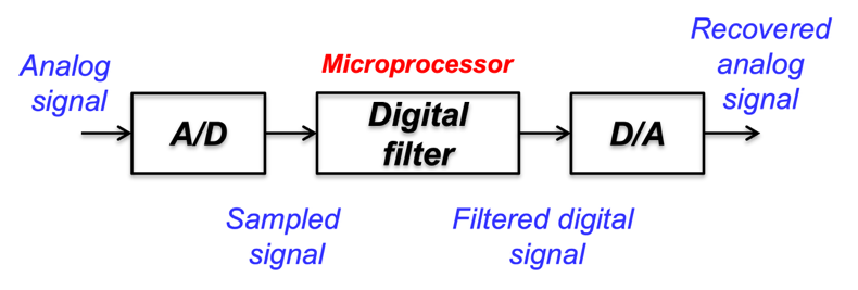
We will address the low-pass digital filter first. Recall that the low-pass analog filter was introduced at the beginning of this section in equation \ref{4.59}. We will represent the digital filter by a \(z\)-transform and implemented as a numerical algorithm executed by the microprocessor. From the equivalence of the Laplace and \(z\)-transforms in Table 4.3, we can see that the corresponding first order digital low-pass filter has the following \(z\)-transform.

\[F_{L1}\left(z\right)=\dfrac{Y(z)}{U(z)}=\dfrac{1-e^{-ω_cT}}{1-e^{-ω_cT}z^{-1}} \label{4.84}\]

where \(ω_c\) is the continuous-time equivalent cutoff frequency, \(T\) is the sample period for the A/D converter, and \(z^{-1}\) is a one-step delay operator.

Note that \(U(z)\) is the original signal and \(Y\left(z\right)\) is the filtered signal in the \(z\)-transform. By the final value theorem of the \(z\)-transform (setting \(z=1\)), we can see that \(F_{L1}\left(1\right)=1\). Recall that the final valve theorem for the Laplace transform sets “\(\mathrm{s}\)” to zero. Therefore, this low-pass digital filter transfer function does have a DC gain equal to one. In order to implement the low-pass filter into an algorithm, we need to develop a calculation formula (algorithm). As a result, the above equation can be reorganized into the following.

\[Y\left(z\right)\left(1-e^{-ω_cT}z^{-1}\right)=\left(1-e^{-ω_cT}\right)U\left(z\right)\to Y\left(z\right)=\left(1-e^{-ω_cT}\right)U\left(z\right)+e^{-ω_cT}z^{-1}Y(z) \label{4.85}\]

The inverse \(z\)-transform of equation \ref{4.85} yields the following.

\[y\left(k\right)=\left(1-e^{-ω_cT}\right)u\left(k\right)+e^{-ω_cT}y(k-1) \label{4.86}\]

Equation \ref{4.86} shows an update logic (algorithm) for filtered signal \(y(k)\) based on the current input signal \(u\left(k\right)\) and the previous estimated signal \(y(k-1)\). We can see that the update logic is a convex combination of the current input \(u(k)\) and previous estimated value \(y(k-1)\). As the cutoff frequency increases, more weight is on the current input \(u(k)\) because \(e^{-ω_cT}\) reduces as \(ω_c\) increases, and vice versa.

One question worth answer is whether there is any correlation between the continuous- and discrete-time filters. Figure 4.45 plots out the frequency responses of both continuous- and discrete-time first order low-pass filters, where the cutoff frequency \(ω_c\) is 5 rad/s with a sample period of \(T=0.002\) (sample frequency of 500 \(Hz\) or 3141.6 rad/s) for the digital filter. Note that the blue-dashed and red-solid lines represent the continuous- and discrete-time filters, respectively.

Applying the Nyquist-Shannon theorem (see Section 4.5), the maximum frequency that can be handled by the digital filter is half of the sample frequency. Here it is 1570.8 rad/s, which is shown in Figure 4.45 as the vertical thin black-line. We can see that as the frequency approaches \(ω_c/2=1570.8\) rad/s, both the magnitude and phase traces diverge from the continuous-time ones, especially for the discrete-time phase response. In summary, at the frequency far away from \(ω_c/2=1570.8\) rad/s, the magnitude and phase responses of both continuous- and discrete-time first order low-pass filters are very close. That is, the digital filter behaves like the continuous-time one. It is important to know the limitation of the digital filter used.

The high-order low-pass filter can also be designed in a manner similar to the first order case and will not be addressed here.

Now, we will discuss digital high-pass filters. They can be considered as all-pass filtered signals minus a low-pass filtered one, as illustrated in Figure 4.46 with a sample transfer function of the first order filter.

The \(z\)-transform of the first order high-pass transfer function can be derived in equation \ref{4.87} based on the architecture shown in Figure 4.46.

\[F_{H1}\left(z\right)=\dfrac{Y(z)}{U(z)}=1-\dfrac{1-e^{-ω_cT}}{1-e^{-ω_cT}z^{-1}}=\dfrac{e^{-ω_cT}(1-z^{-1})}{1-e^{-ω_cT}z^{-1}} \label{4.87}\]

From the filter transfer function shown in equation \ref{4.87}, the inverse \(z\)-transform yields the following high-pass filter calculation logic that can be implemented in the form of software.

\[y\left(k\right)=e^{-ω_cT}y\left(k-1\right)+e^{-ω_cT}\left[u(k)-u(k-1)\right] \label{4.88}\]

However, for extremely fast applications, FPGA (field programmable gate arrays) silicon is often used for implementing digital filters with certain cost [11]. Both band-pass and band-kill filters can be designed using the low- and high-pass filters with the scheme of continuous-time filters presented in the beginning of this section. Therefore, we will not address these two-filter design schemes again in the discrete-time case.

Example 4.15

For this example, we will study the effect of a first order digital filter on a random digital signal generated by the MATLAB command randn with \(2^{14}\) points and variance equal to one. The original and FFT (fast Fourier transform) response are plotted in Figure 4.47, where the first 20-second time response is plotted (see the left chart) and its FFT is plotted (see the right chart). We assume that the digital signal has a sample period of \(T=0.002\) second (500 Hz), leading to the highest frequency component of 250 \(Hz\) (or 1570.8 rad/s) from FFT. We can also see that the FFT frequency response has a constant averaged magnitude with an oscillation magnitude that increases as frequency goes up.

Next, we will study the behavior of a first order digital filter equivalent to a given continuous-time filter with the transfer function below.

\[ F_{L1}\left(s\right)=\dfrac{a}{s+a}, \ a=5 \label{4.89}\]

With the sample period of \(T=0.002\) second, we have the following \(z\)-transform of the digital low-pass filter.

\[ F_{L1}\left(z\right)=\dfrac{1-b}{1-bz^{-1}}, \ b=e^{aT}=0.9512 \label{4.90}\]

Now, we will look at the frequency response of the first order digital filter based on FFT so that we can compare it with the result from Figure 4.45. Let \(U(z)\) and \(Y(z)\) be the fast Fourier transforms of the random signal generated by MATLAB and the time response of the filtered signal below.

\[ U\left(z\right)=FFT\left(randn\left(2^{14},1\right)\right), \ Y\left(z\right)=FFT\left(by\left(k-1\right)+bu(k)\right) \label{4.91}\]

We can estimate the filter frequency response numerically as below; see reference [23] for its derivation.

\[ \hat{F}\left(z\right)=Y./U(z) \label{4.92}\]

where “\(./\)” is a point-wise division operation. Figure 4.48 above shows the frequency response calculated based on the FFT result in equation \ref{4.91} with the MATLAB command sys=frd(Z, omega), where \(omega=ω\) is the frequency vector. It can be seen that the frequency response is similar to that in Figure 4.45.

Figure 4.49 plots the frequency response \(Y(z)\) directly. The cutoff frequency is around \(5\) rad/s. Because the input signal is a random signal with uniform spectrum, the cutoff frequency of the filtered frequency response represents the filtered one. In addition, 20 dB decay of the frequency response is also observed, indicating a first order filter is used.

---