Opening the book…
- Finite Statistics with Student \(t\) distribution
- Normal distribution assumes an infinite population, but only limited samples are available for calculating the mean and variance of a sample set.
- Sample mean \[ \bar{x} = \frac{1}{N} \sum_{i=1}^{N} x_{i} \] \[ \bar{x} \neq x' \ \mathrm{explicitly} \]
- Sample variance \[ S_{x}^{2} = \frac{1}{N-1}\sum_{i=1}^{N}(x_{i}-\bar{x})^{2} \]
- Since another statistical term was used in \(S_{x}\), the degree of freedom is considered \[\nu = N-c\] where \(N\) is the number of samples and \(c\) is the number of statistical constraints used in calculations.
- If accidentally substituting sample statistics into Normal distribution \[ p(x) = \frac{1}{S_{x}\sqrt{2\pi}}\mathrm{e}^{\frac{-(x-\bar{x})^{2}}{2S_{x}^{2}}} \] then
- Comparison of the distribution of normal (blue) and finite statistics (red)
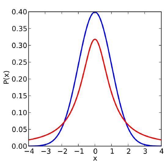
- An overestimate of probability near sample mean
- Underestimates the probability far from the tail
- More complex function so two-sided Table format is provided
- Comparison of the distribution of normal (blue) and finite statistics (red)
- Normalizing the \(t\) variable (similar to \(z_{1}\))
- Non-dimensional term \[ t = \frac{x-\bar{x}}{S_{x}} \] depends on two parameters
- \(\nu\) degree of freedom (i.e., # of samples)
- \(P\) confidence interval of probability
- Method of prediction of next selection of random variable \[ x_{N+1} = \bar{x} \pm t_{\nu,P}S_{x}\ (\%\ P)\]
- Same confidence interval \(\%\ P\) but fewer samples increases range of uncertainty
- Same sample size but smaller \(\%\ P\) reduces range of uncertainty
- As \(N\rightarrow \infty\), then \(t_{\nu, P}\rightarrow z_{p}\) since the sample statistics approach infinite terms
- Non-dimensional term \[ t = \frac{x-\bar{x}}{S_{x}} \] depends on two parameters
- Example
Example of finite version: Consider the same capacitors but mean (\(\bar{x} = 145\ \mu\)F) and standard deviation (\(S_{x} = 33\ \mu\)F) statistics are determined from 31 samples.
- What is expected value of the next capacitor with 95% confidence?
- How would fewer data points \(N<31\) affect that range for the prediction?
- Answer
-
From the set of \(\nu = N - 1 = 30\) and confidence interval, the \(t_{30,95\%} = 2.042\). Therefore \[x_{32} = 145 \pm 2.042(33) = 77.6 \longleftrightarrow 212.4\ \mu\mathrm{F}\]
If the same mean and standard deviation statistics were collected from \(N=24\) data points, \(t_{23,95\%} = 2.069\) then the results would indicate \[ 76.7 < x_{25} < 213.3\ \mu\mathrm{F}\]
- Using the Standard Deviation of the Means
- The sample statistics \(\bar{x}\) and \(S_{x}\) provide insight on the true properties \(x'\) and \(\sigma\), respectively.
- Using the \(N\) samples, the central limit theorem offers a range on the prediction of the true mean: \[x' = \bar{x} \pm t_{\nu,P}S_{\bar{x}} \] where \[S_{\bar{x}} = \frac{S_{x}}{\sqrt{N}}\]
- Note the difference between the next measurement versus and indication of the true mean value with the confidence interval.
- Offers an uncertainty of \(x'\) from the statistics instead of the sensor
-
From the prior example, how large is uncertainty of the true mean value from 24 samples at 99.5\% confidence?
- Answer
-
The \(t\) multiplier is found from \(t_{23,99.5\%} = 3.104 \). Hence, the range of the true mean would be \[x' = 145 \pm 3.104\left(\frac{33}{\sqrt{24}}\right) = 145 \pm 20.91\ \mu\mathrm{F}\]
The width of the uncertainty decreases as the confidence level \(\% P\) similarly decreases.
- Normal distribution assumes an infinite population, but only limited samples are available for calculating the mean and variance of a sample set.
- Design of Experiments

7.4: Analysis with finite statistics is shared under a CC BY-NC 4.0 license and was authored, remixed, and/or curated by LibreTexts.
The book could not be loaded just now.