Opening the book…
Table 16.3.1 , at the bottom of this appendix, gives the proportion, P, of the area under a normal distribution curve that lies to the right of a deviation, z
\[z = \frac {X -\mu} {\sigma} \nonumber\]
where X is the value for which the deviation is defined, \(\mu\) is the distribution’s mean value and \(\sigma\) is the distribution’s standard deviation. For example, the proportion of the area under a normal distribution to the right of a deviation of 0.04 is 0.4840 (see entry in red in the table), or 48.40% of the total area (see the area shaded blue in Figure 16.3.1 ). The proportion of the area to the left of the deviation is 1 – P. For a deviation of 0.04, this is 1 – 0.4840, or 51.60%.
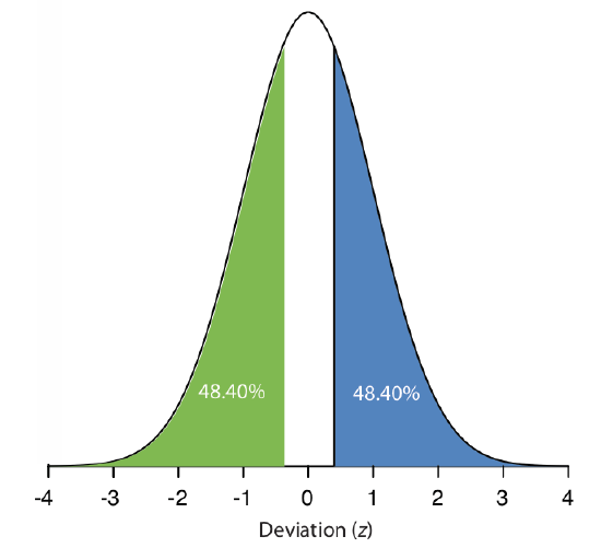
Figure 16.3.1 . Normal distribution curve showing the area under a curve greater than a deviation of +0.04 (blue) and with a deviation less than –0.04 (green).
When the deviation is negative—that is, when X is smaller than \(\mu\)—the value of z is negative. In this case, the values in the table give the area to the left of z. For example, if z is –0.04, then 48.40% of the area lies to the left of the deviation (see area shaded green in Figure 16.3.1 .
To use the single-sided normal distribution table, sketch the normal distribution curve for your problem and shade the area that corresponds to your answer (for example, see Figure 16.3.2 , which is for Example 4.4.2).
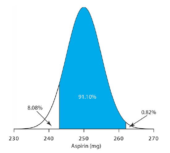
This divides the normal distribution curve into three regions: the area that corresponds to our answer (shown in blue), the area to the right of this, and the area to the left of this. Calculate the values of z for the limits of the area that corresponds to your answer. Use the table to find the areas to the right and to the left of these deviations. Subtract these values from 100% and, voilà, you have your answer.
| z | 0.00 | 0.01 | 0.02 | 0.03 | 0.04 | 0.05 | 0.06 | 0.07 | 0.08 | 0.09 |
| 0.0 | 0.5000 | 0.4960 | 0.4920 | 0.4880 | 0.4840 | 0.4801 | 0.4761 | 0.4721 | 0.4681 | 0.4641 |
| 0.1 | 0.4602 | 0.4562 | 0.4522 | 0.4483 | 0.4443 | 0.4404 | 0.4365 | 0.4325 | 0.4286 | 0.4247 |
| 0.2 | 0.4207 | 0.4168 | 0.4129 | 0.4090 | 0.4502 | 0.4013 | 0.3974 | 0.3396 | 0.3897 | 0.3859 |
| 0.3 | 0.3821 | 0.3783 | 0.3745 | 0.3707 | 0.3669 | 0.3632 | 0.3594 | 0.3557 | 0.3520 | 0.3483 |
| 0.4 | 0.3446 | 0.3409 | 0.3372 | 0.3336 | 0.3300 | 0.3264 | 0.3228 | 0.3192 | 0.3156 | 0.3121 |
| 0.5 | 0.3085 | 0.3050 | 0.3015 | 0.2981 | 0.2946 | 0.2912 | 0.2877 | 0.2843 | 0.2810 | 0.2776 |
| 0.6 | 0.2743 | 0.2709 | 0.2676 | 0.2643 | 0.2611 | 0.2578 | 0.2546 | 0.2514 | 0.2483 | 0.2451 |
| 0.7 | 0.2420 | 0.2389 | 0.2358 | 0.2327 | 0.2296 | 0.2266 | 0.2236 | 0.2206 | 0.2177 | 0.2148 |
| 0.8 | 0.2119 | 0.2090 | 0.2061 | 0.2033 | 0.2005 | 0.1977 | 0.1949 | 0.1922 | 0.1894 | 0.1867 |
| 0.9 | 0.1841 | 0.1814 | 0.1788 | 0.1762 | 0.1736 | 0.1711 | 0.1685 | 0.1660 | 0.1635 | 0.1611 |
| 1.0 | 0.1587 | 0.1562 | 0.1539 | 0.1515 | 0.1492 | 0.1469 | 0.1446 | 0.1423 | 0.1401 | 0.1379 |
| 1.1 | 0.1357 | 0.1335 | 0.1314 | 0.1292 | 0.1271 | 0.1251 | 0.1230 | 0.1210 | 0.1190 | 0.1170 |
| 1.2 | 0.1151 | 0.1131 | 0.1112 | 0.1093 | 0.1075 | 0.1056 | 0.1038 | 0.1020 | 0.1003 | 0.0985 |
| 1.3 | 0.0968 | 0.0951 | 0.0934 | 0.0918 | 0.0901 | 0.0885 | 0.0869 | 0.0853 | 0.0838 | 0.0823 |
| 1.4 | 0.0808 | 0.0793 | 0.0778 | 0.0764 | 0.0749 | 0.0735 | 0.0721 | 0.0708 | 0.0694 | 0.0681 |
| 1.5 | 0.0668 | 0.0655 | 0.0643 | 0.0630 | 0.0618 | 0.0606 | 0.0594 | 0.0582 | 0.0571 | 0.0559 |
| 1.6 | 0.0548 | 0.0537 | 0.0526 | 0.0516 | 0.0505 | 0.0495 | 0.0485 | 0.0475 | 0.0465 | 0.0455 |
| 1.7 | 0.0466 | 0.0436 | 0.0427 | 0.0418 | 0.0409 | 0.0401 | 0.0392 | 0.0384 | 0.0375 | 0.0367 |
| 1.8 | 0.0359 | 0.0351 | 0.0344 | 0.0336 | 0.0329 | 0.0322 | 0.0314 | 0.0307 | 0.0301 | 0.0294 |
| 1.9 | 0.0287 | 0.0281 | 0.0274 | 0.0268 | 0.0262 | 0.0256 | 0.0250 | 0.0244 | 0.0239 | 0.0233 |
| 2.0 | 0.0228 | 0.0222 | 0.0217 | 0.0212 | 0.0207 | 0.0202 | 0.0197 | 0.0192 | 0.0188 | 0.0183 |
| 2.1 | 0.0179 | 0.0174 | 0.0170 | 0.0166 | 0.0162 | 0.0158 | 0.0154 | 0.0150 | 0.0146 | 0.0143 |
| 2.2 | 0.0139 | 0.0136 | 0.0132 | 0.0129 | 0.0125 | 0.0122 | 0.0119 | 0.0116 | 0.0113 | 0.0110 |
| 2.3 | 0.0107 | 0.0104 | 0.0102 | 0.00964 | 0.00914 | 0.00866 | ||||
| 2.4 | 0.00820 | 0.00776 | 0.00734 | 0.00695 | 0.00657 | |||||
| 2.5 | 0.00621 | 0.00587 | 0.00554 | 0.00523 | 0.00494 | |||||
| 2.6 | 0.00466 | 0.00440 | 0.00415 | 0.00391 | 0.00368 | |||||
| 2.7 | 0.00347 | 0.00326 | 0.00307 | 0.00289 | 0.00272 | |||||
| 2.8 | 0.00256 | 0.00240 | 0.00226 | 0.00212 | 0.00199 | |||||
| 2.9 | 0.00187 | 0.00175 | 0.00164 | 0.00154 | 0.00144 | |||||
| 3.0 | 0.00135 | |||||||||
| 3.1 | 0.000968 | |||||||||
| 3.2 | 0.000687 | |||||||||
| 3.3 | 0.000483 | |||||||||
| 3.4 | 0.000337 | |||||||||
| 3.5 | 0.000233 | |||||||||
| 3.6 | 0.000159 | |||||||||
| 3.7 | 0.000108 | |||||||||
| 3.8 | 0.0000723 | |||||||||
| 3.9 | 0.0000481 | |||||||||
| 4.0 | 0.0000317 |
This page titled 7.3: Single-Sided Normal Distribution was last modified on Sun, 11 Feb 2024 02:10:49 GMT and is shared under a CC BY-NC-SA 4.0 license and was authored, remixed, and/or curated by David Harvey.
The book could not be loaded just now.