Opening the book…
The problem is that STOs do not perform well with numerical integration methods: in most cases, numerical integrals involving these functions requires very large grid sizes and limits. To overcome this problem, computational chemists have developed Gaussian-type orbitals (GTOs), which can be numerically integrated in a much more efficient manner. Some integrals become solvable analytically, and other multidimensional integrals can be transformed into products of single-dimensional ones, dramatically reducing the computational cost for evaluating them.
Gaussian Type Orbitals (GTO)
Although any basis set that sufficiently spans the space of electron distribution could be used, the concept of Molecular Orbitals as Linear Combinations of Atomic Orbitals (LCAO) suggests a very natural set of basis functions: AO-type functions centered on each nuclei. One obvious choice are the exact hydrogen AO's, known as Slater-type orbitals (STO) -describing the radial component of the functions. However, the computation of the integrals is greatly simplified by using Gaussian-type orbitals (GTO) for basis functions.
While the STO basis set was an improvement over hydrogenic orbitals in terms of computational efficiency, representing the STOs with Gaussian functions produced further improvements that were needed to accurately describe molecules. The GTOs are most frequently expressed in Cartesian coordinates:
\[\ket{\phi^{GTO}_{abc}(x,y,z;\alpha)} = Ne^{-\alpha r^2}(x-x_0)^a(y-y_0)^b(z-z_0)^c, \label{4} \]
where \(\alpha\) is the shape term that can be optimized, \(x\), \(y\), and \(z\) are Cartesian coordinates for an electron in an orbital whose center is located at position \((x_0,y_0,z_0)\), and \(a\), \(b\), and \(c\) are nonnegative integers that serve a similar function to the \(\ell\) and \(m\) quantum numbers for selecting the shape of the orbital. An orbital with angular momentum \(\ell\) is created by choosing \(a + b + c = \ell\). For instance, a \(p_x\) orbital shape can be approximated by letting \(a=1\), \(b=0\), and \(c=0\), and a \(d_{zz}\) orbital by \(a=0\), \(b=0\), and \(c=2\). Once again \(N\) is a normalization constant, and \(r = \sqrt{x^2 + y^2 + z^2}\).
One significant point to note about Cartesian Gaussian functions is that when \(\ell \geq 2\), there are more Cartesian functions than atomic orbitals with the same value of \(\ell\). As a simple example, when \(\ell = 2\) (i.e., a \(d\) orbital), there are 5 spherical harmonic functions: those with \(m = 2, 1, 0, -1\), and \(-2\). However, there are 6 ways to make Cartesian Gaussian functions with \(\ell=2\): \(x^2\), \(y^2\), \(z^2\), \(xy\), \(yz\), and \(xz\). This means that if a set of Cartesian functions is used to represent \(d\) orbitals, the set of 6 functions is contaminated by a contribution from one or more orbitals of different \(\ell\) (in this case, the linear combination of Cartesian Gaussians \(d_{xx} + d_{yy} + d_{zz}\) is actually an \(s\)-type orbital with \(\ell=0\)). In general, the number of Cartesian functions that can be formed for a given \(\ell\) is \((\ell+1)(\ell+2)/2\), while the number of “spherical harmonic” Gaussian functions is \(2\ell+1\). Nevertheless, it is possible to apply a mathematical transformation to the Cartesian Gaussian functions to extract combinations equivalent to the corresponding spherical-harmonic Gaussian functions, so for the purposes of this course, we will assume that this is always done. Therefore, we will assume that if a basis set includes a set of \(d\) functions, for instance, the number of functions in the set is 5, not 6.
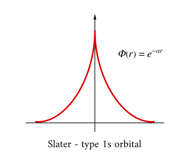
The biggest limitation of GTOs is that they do not have quite the right shape close to the nucleus (near \(r=0\)): the exponential term goes as \(-\alpha r^2\) rather than \(-\alpha r\). The “cusp” that is obtained by an exponential with an \(r^{-1}\) dependence is not well reproduced by an exponential function that goes as \(r^{-2}\). ( Figure \(\PageIndex{1}\)).

Multiple Gaussian Representation
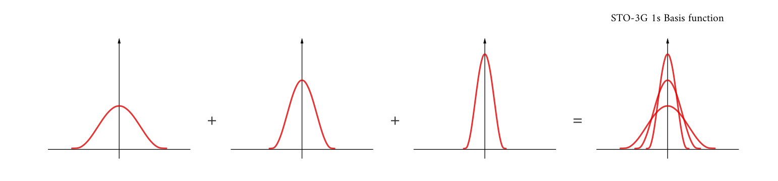
This can be partially overcome by using a linear combination of GTOs to approximate an STO; these are called “contracted” basis functions. One of the first of these basis sets to be developed was the \(STO-NG\) family, in which a single STO is expressed as a contracted function involving \(N\) GTOs (see Figure \(\PageIndex{2}\)):
\[\ket{\psi_i^{\text{STO-NG}}} = \sum_n^N d_{in}\ket{\phi^{GTO}(\alpha_{in})} \label{chap:mot:eq:stong} \]
where \(i\) is the type of STO being approximated (eg \(1s\)), \(d_{in}\) are the optimized expansion coefficients for each GTO in the linear combination for orbital \(i\), and \(\alpha_{in}\) are the optimized \(\alpha\) terms for each GTO. The \(d\) and \(\alpha\) terms are varied to maximize overlap with the corresponding STO; tabulations of these are available, though they’re not difficult to calculate. When these STO-\(N\)G basis functions are used in a molecular calculation, the \(d\) and \(\alpha\) coefficients are not adjusted any further; once those constants are set, the entire linear combination \(\ket{\psi_i^{\text{STO-NG}}}\) acts like a single STO atomic orbital.
The linear combination in Equation \ref{chap:mot:eq:stong} is not optimized in the energy variational calculation, but rather is frozen and treated as a single function. The linear combination of primitive Gaussian functions is called a contracted Gaussian function.
Although multiple GTOs are required to approximate a single STO, electronic structure calculations involving GTOs are much faster than with STOs. All overlap integrals can be evaluated analytically, and for most other types of integrals (Coulomb and exchange integrals, both one-electron and two-electron), the full 3D or 6D integral can be split into a product of 3 or 6 one-dimensional integrals. For a 6D integral with 100 grid points, an STO may require \(100^6\) function evaluations, while the same integral over a single GTO may require only 600. Moreover, there are several clever quadrature strategies for integrals involving products of Gaussians which reduce the number of quadrature points required for accurate evaluation. Thus, despite the need for using a combination of several GTOs to create an orbital function of comparable quality to a single STO, a calculation involving GTOs can achieve the same accuracy as one involving STOs in a much shorter time.

For this reason, almost all modern electronic structure calculations are performed using basis sets built from combinations of GTOs. Basis set development is undertaken by a variety of theoretical chemists in an effort to make calculations of certain types of molecules or molecular properties more efficient; these groups perform tedious optimizations of various parameters (\(\alpha\), \(N\), \(d\), etc.) for each orbital representing each atom in order to reproduce experimentally measured quantities or quantities calculated at very high levels of theory. The results of these benchmarks are published, and the optimized coefficients are made available to standard quantum chemical packages. One of the main sources for obtaining and learning about basis sets is the Basis Set Exchange website (https://bse.pnl.gov); most basis sets used in the chemical literature have been deposited there.
Basis Notation
Many types of basis sets exist, and their designations (e.g., 6-311++G\(^{**}\), aug-cc-pCV5Z, etc.) can look like alphabet soup to the uninitiated. Nevertheless, with many electronic structure packages, choosing a basis set is often as simple as typing in its name; most common basis sets are pre-loaded into these programs, and if you require a basis set that is not already there, the Basis Set Exchange website has many available in a variety of input formats. Because of the ease of choosing a basis set, it can be tempting to overlook the details, but knowledge of what kinds of functions are included in different classes of basis sets, as well as which basis sets are optimal for what types of molecular problems, can save a lot of time. Here we will introduce a couple of commonly used classes of basis functions, along with some of the terminology used to describe them.
Gaussian basis sets are identified by abbreviations such as N-MPG*. N is the number of Gaussian primitives used for each inner-shell orbital. The hyphen indicates a split-basis set where the valence orbitals are double zeta. The M indicates the number of primitives that form the large zeta function (for the inner valence region), and P indicates the number that form the small zeta function (for the outer valence region). G identifies the set a being Gaussian. The addition of an asterisk to this notation means that a single set of Gaussian 3d polarization functions (discussed elsewhere) is included. A double asterisk means that a single set of Gaussian 2p functions is included for each hydrogen atom.
For example, 3G means each STO is represented by a linear combination of three primitive Gaussian functions. 6-31G means each inner shell (1s orbital) STO is a linear combination of 6 primitives and each valence shell STO is split into an inner and outer part (double zeta) using 3 and 1 primitive Gaussians, respectively (see Table \(\PageIndex{1}\) for other examples).
| Basis set | # functions | Basis set | # functions | Basis set | # functions | ||
|---|---|---|---|---|---|---|---|
| STO-3G | 5 | 6-31G | 9 | 6-31 1G | 13 | ||
| 3-21G | 9 | 6-31G* | 15 | 6-311G* | 18* | ||
| 4-31G | 9 | 6-31+G* | 19 | 6-311+G* | 22* |
The 1s Slater-type orbital \(S_1 (r) = \sqrt {4 \zeta _1 e^{-\zeta _1 r}}\) with \(\zeta _1 = 1.24 \) is represented as a sum of three primitive Gaussian functions,
\[S_G (r) = \sum _{j=1}^3 C_j e^{-\alpha _j r^2} \nonumber \]
This sum is the contracted Gaussian function for the STO.
- Make plots of the STO and the contracted Gaussian function on the same graph so they can be compared easily. All distances should be in units of the Bohr radius. Use the following values for the coefficients, C, and the exponential parameters, \(\alpha\).
index j \(\alpha _j\) \(C_j\) 1 0.1688 0.4 2 0.6239 0.7 3 3.425 1.3 - Change the values of the coefficients and exponential parameters to see if a better fit can be obtained.
- Comment on the ability of a linear combination of Gaussian functions to accurately describe a STO.
Summary
STOs are computationally difficult and it was later realized by Frank Boys that these Slater-type orbitals could in turn be approximated as linear combinations of Gaussian orbitals instead. Because it is easier to calculate overlap and other integrals with Gaussian basis functions, this led to huge computational savings
12.4: Gaussian Basis Sets is shared under a CC BY-NC-SA 4.0 license and was authored, remixed, and/or curated by LibreTexts.
The book could not be loaded just now.